Part 3. Compare simulations

from pathlib import Path

%matplotlib inline
import matplotlib.pyplot as plt

plt.rc("figure", dpi=80)

def get_values(sim):
    N = sim.params.N
    Uc = sim.params.forcing.milestone.movement.periodic_uniform.speed
    Dc = sim.params.forcing.milestone.objects.diameter
    Lf = sim.params.forcing.milestone.movement.periodic_uniform.length

    Fhc = Uc / (N * Dc)
    Rec = Uc * Dc / sim.params.nu_2

    period = sim.forcing.get_info()["period"]
    t_statio = period
    averages = sim.output.spatial_means.get_dimless_numbers_averaged(
        tmin=t_statio
    )

    U2 = averages["dimensional"]["Uh2"]
    epsK = averages["dimensional"]["epsK"]
    Gamma = averages["Gamma"]
    Fh = averages["Fh"]
    R2 = averages["R2"]
    R4 = averages["R4"]

    return N, Uc, Dc, Lf, Fhc, Rec, U2, epsK, Gamma, Fh, R2, R4

import fluidsim as fls

path_dir_data = Path(fls.FLUIDSIM_PATH) / "tutorial_parametric_study"
path_runs = sorted(path_dir_data.glob("*"), key=lambda p: p.name)
[p.name for p in path_runs]

['ns3d.strat_144x144x48_V4.5x4.5x1.5_N0.2_Lf3.5_U0.01_D0.5_2021-10-05_15-35-47',
 'ns3d.strat_144x144x48_V4.5x4.5x1.5_N0.2_Lf3.5_U0.02_D0.5_2021-10-05_16-12-36',
 'ns3d.strat_144x144x48_V4.5x4.5x1.5_N0.2_Lf3.5_U0.04_D0.5_2021-10-05_16-49-31',
 'ns3d.strat_144x144x48_V4.5x4.5x1.5_N0.2_Lf3.5_U0.06_D0.5_2021-10-05_17-25-48',
 'ns3d.strat_144x144x48_V4.5x4.5x1.5_N0.2_Lf3.5_U0.08_D0.5_2021-10-05_18-01-23']

Compare simulations with Pandas

import numpy as np
from pandas import DataFrame

# fmt: off
columns = ["N", "Uc", "Dc", "Lf", "Fhc", "Rec", "U2", "epsK", "Gamma", "Fh", "R2", "R4"]
# fmt: on

values = []
for path in path_runs:
    sim = fls.load(path, hide_stdout=True)
    values.append(get_values(sim))

df = DataFrame(values, columns=columns)
df["min_R"] = np.array([df.R2, df.R4]).min(axis=0)
df

	N	Uc	Dc	Lf	Fhc	Rec	U2	epsK	Gamma	Fh	R2	R4	min_R
0	0.2	0.01	0.5	3.5	0.1	5000.0	0.000030	5.564985e-08	0.300576	0.009451	1.391246	0.170957	0.170957
1	0.2	0.02	0.5	3.5	0.2	10000.0	0.000109	3.917927e-07	0.468731	0.018019	9.794817	2.204561	2.204561
2	0.2	0.04	0.5	3.5	0.4	20000.0	0.000419	2.834370e-06	0.618684	0.034420	70.859251	30.298269	30.298269
3	0.2	0.06	0.5	3.5	0.6	30000.0	0.000914	8.980284e-06	0.629455	0.049961	224.507095	139.360780	139.360780
4	0.2	0.08	0.5	3.5	0.8	40000.0	0.001652	2.199885e-05	0.561550	0.067149	549.971217	463.932956	463.932956

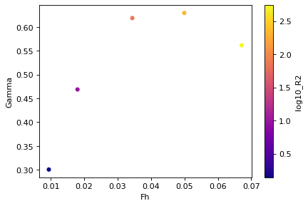
df["log10_R2"] = np.log10(df.R2)
fig, ax = plt.subplots()
df.plot.scatter(ax=ax, x="Fh", y="Gamma", c="log10_R2", cmap="plasma");

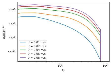
A figure with data from different simulations

fig, ax = plt.subplots()

for path in path_runs:
    sim = fls.load(path, hide_stdout=True)
    period = sim.forcing.get_info()["period"]
    data = sim.output.spectra.load1d_mean(tmin=period)
    spectrum = data["spectra_vx_kx"]
    kx = data["kx"]
    ax.loglog(
        kx,
        spectrum * kx ** (5 / 3),
        label=f"U = {sim.params.forcing.milestone.movement.periodic_uniform.speed} m/s",
    )

ax.set_xlabel("$k_x$")
ax.set_ylabel("$E_x(k_z) {k_z}^{5/3}$")
plt.legend();

compute mean of spectra
tmin =  800.502 ; tmax =  1600.67
imin =      100 ; imax =      200
compute mean of spectra
tmin =  400.051 ; tmax =  800.132
imin =      100 ; imax =      200
compute mean of spectra
tmin =  200.093 ; tmax =  400.025
imin =      100 ; imax =      200
compute mean of spectra
tmin =  133.342 ; tmax =  266.703
imin =      101 ; imax =      201
compute mean of spectra
tmin =  100.004 ; tmax =  200.024
imin =      100 ; imax =      200