Test case: Taylor-Green vortex initial value problem
This is can be a resource intensive test depending on the number of resolution of the simulation. It is preferrable to execute this with MPI parallelization. Ideally we would do this as follows from the root of the fluidsim repository.
mpirun -np $(nproc) python doc/test_cases/Taylor_Green_vortices/run_simul.py
Preparation
Instead we are executing the script within a IPython kernel inside a Jupyter notebook, we require ipyparallel backend launched in the background by running:
ipcluster start -n $(nproc) --engines=MPIEngineSetLauncher
or from another IPython kernel
!{sys.executable} -m ipyparallel.apps.ipclusterapp start -n $(nproc) --engines=MPIEngineSetLauncher
And then we connect to the MPI engine.
import ipyparallel as ipp

rc = ipp.Client()
dview = rc[:]
Afterwards, we will execute all cells in parallel so we always need to add the magic command %%px.
Initialize parameters
The following script was loaded by running %load doc/test_cases/Taylor_Green_vortices/run_simul.py and slightly modified to use a higher resolution (nx).
%%px
"""Taylor-Green Vortex at Re = 1600
===================================

https://www.grc.nasa.gov/hiocfd/wp-content/uploads/sites/22/case_c3.3.pdf


"""

import numpy as np

from fluidsim.solvers.ns3d.solver import Simul

params = Simul.create_default_params()

Re = 1600
V0 = 1.0
L = 1
params.nu_2 = V0 * L / Re

params.init_fields.type = "in_script"

params.time_stepping.t_end = 20.0 * L / V0

nx = 96
params.oper.nx = params.oper.ny = params.oper.nz = nx
lx = params.oper.Lx = params.oper.Ly = params.oper.Lz = 2 * np.pi * L

params.output.periods_save.phys_fields = 4
params.output.periods_save.spatial_means = 0.2
params.output.periods_save.spectra = 0.5

sim = Simul(params)

X, Y, Z = sim.oper.get_XYZ_loc()

vx = V0 * np.sin(X / L) * np.cos(Y / L) * np.cos(Z / L)
vy = -V0 * np.cos(X / L) * np.sin(Y / L) * np.cos(Z / L)
vz = sim.oper.create_arrayX(value=0)

sim.state.init_statephys_from(vx=vx, vy=vy, vz=vz)

sim.state.statespect_from_statephys()
sim.state.statephys_from_statespect()
[stdout:0]
*************************************
Program fluidsim
Manual initialization of the fields is selected. Do not forget to initialize them.
sim:                <class 'fluidsim.solvers.ns3d.solver.Simul'>
sim.oper:           <class 'fluidsim.operators.operators3d.OperatorsPseudoSpectral3D'>
sim.output:         <class 'fluidsim.solvers.ns3d.output.Output'>
sim.state:          <class 'fluidsim.solvers.ns3d.state.StateNS3D'>
sim.time_stepping:  <class 'fluidsim.solvers.ns3d.time_stepping.TimeSteppingPseudoSpectralNS3D'>
sim.init_fields:    <class 'fluidsim.solvers.ns3d.init_fields.InitFieldsNS3D'>

solver ns3d, RK4 and parallel (6 proc.)
type fft: fluidfft.fft3d.mpi_with_fftwmpi3d
nx =     96 ; ny =     96 ; nz =     96
Lx = 2pi ; Ly = 2pi ; Lz = 2pi
path_run =
/scratch/avmo/tmp/ns3d_96x96x96_V2pix2pix2pi_2019-01-15_14-17-34
init_fields.type: in_script
To preview the initialization one could do the following before time stepping. This is only useful to plot fields, and only recommended when run sequentially.
%matplotlib inline
sim.output.init_with_initialized_state()
sim.output.phys_fields.plot(equation=f'x={{sim.oper.Lx/4}}')
Run the simulation
%%px --no-verbose
sim.time_stepping.start()
[stdout:0]
Initialization outputs:
sim.output.phys_fields:       <class 'fluidsim.base.output.phys_fields3d.PhysFieldsBase3D'>
sim.output.spatial_means:     <class 'fluidsim.solvers.ns3d.output.spatial_means.SpatialMeansNS3D'>
sim.output.spectra:           <class 'fluidsim.solvers.ns3d.output.spectra.SpectraNS3D'>

Memory usage at the end of init. (equiv. seq.): 1285.1171875 Mo
Size of state_spect (equiv. seq.): 21.676032 Mo
*************************************
Beginning of the computation
save state_phys in file state_phys_t000.000.nc
    compute until t =         20
it =      0 ; t =          0 ; deltat  =   0.032725
              energy = 1.250e-01 ; Delta energy = +0.000e+00

it =     32 ; t =    1.00953 ; deltat  =   0.030018
              energy = 1.245e-01 ; Delta energy = -4.897e-04
              estimated remaining duration =       345 s
it =     67 ; t =    2.02202 ; deltat  =   0.027502
              energy = 1.239e-01 ; Delta energy = -6.092e-04
              estimated remaining duration =       356 s
it =    106 ; t =    3.02963 ; deltat  =   0.025238
              energy = 1.230e-01 ; Delta energy = -9.115e-04
              estimated remaining duration =       383 s
save state_phys in file state_phys_t004.016.nc
it =    145 ; t =    4.04169 ; deltat  =    0.02493
              energy = 1.214e-01 ; Delta energy = -1.636e-03
              estimated remaining duration =       356 s
it =    193 ; t =    5.04479 ; deltat  =   0.019722
              energy = 1.162e-01 ; Delta energy = -5.187e-03
              estimated remaining duration =       407 s
it =    243 ; t =    6.04514 ; deltat  =   0.019253
              energy = 1.060e-01 ; Delta energy = -1.014e-02
              estimated remaining duration =       396 s
it =    293 ; t =    7.05723 ; deltat  =   0.018782
              energy = 9.229e-02 ; Delta energy = -1.373e-02
              estimated remaining duration =       365 s
save state_phys in file state_phys_t008.027.nc
it =    348 ; t =    8.06488 ; deltat  =   0.019995
              energy = 7.645e-02 ; Delta energy = -1.585e-02
              estimated remaining duration =       375 s
it =    391 ; t =    9.08234 ; deltat  =   0.028734
              energy = 6.253e-02 ; Delta energy = -1.392e-02
              estimated remaining duration =       262 s
it =    426 ; t =    10.0915 ; deltat  =   0.030125
              energy = 5.373e-02 ; Delta energy = -8.791e-03
              estimated remaining duration =       202 s
it =    458 ; t =    11.1164 ; deltat  =    0.03378
              energy = 4.758e-02 ; Delta energy = -6.154e-03
              estimated remaining duration =       160 s
save state_phys in file state_phys_t012.047.nc
it =    489 ; t =    12.1465 ; deltat  =   0.033096
              energy = 4.283e-02 ; Delta energy = -4.752e-03
              estimated remaining duration =       142 s
it =    518 ; t =    13.1745 ; deltat  =   0.036405
              energy = 3.904e-02 ; Delta energy = -3.784e-03
              estimated remaining duration =       111 s
it =    546 ; t =    14.2052 ; deltat  =    0.03635
              energy = 3.584e-02 ; Delta energy = -3.206e-03
              estimated remaining duration =        91 s
it =    574 ; t =    15.2427 ; deltat  =   0.038787
              energy = 3.305e-02 ; Delta energy = -2.787e-03
              estimated remaining duration =      74.3 s
save state_phys in file state_phys_t016.051.nc
it =    599 ; t =    16.2651 ; deltat  =   0.043076
              energy = 3.064e-02 ; Delta energy = -2.414e-03
              estimated remaining duration =      53.5 s
it =    622 ; t =    17.2665 ; deltat  =   0.043052
              energy = 2.853e-02 ; Delta energy = -2.110e-03
              estimated remaining duration =      36.9 s
it =    646 ; t =    18.2694 ; deltat  =   0.041138
              energy = 2.668e-02 ; Delta energy = -1.847e-03
              estimated remaining duration =      24.8 s
it =    671 ; t =    19.2979 ; deltat  =   0.041138
              energy = 2.501e-02 ; Delta energy = -1.666e-03
              estimated remaining duration =      10.2 s
Computation completed in  399.654 s
path_run =
/scratch/avmo/tmp/ns3d_96x96x96_V2pix2pix2pi_2019-01-15_14-17-34
save state_phys in file state_phys_t020.030.nc
move result directory in directory:
/scratch/avmo/data/ns3d_96x96x96_V2pix2pix2pi_2019-01-15_14-17-34
%%px -t 0
sim.output.path_run
Out[0:3]: '/scratch/avmo/data/ns3d_96x96x96_V2pix2pix2pi_2019-01-15_14-17-34'
Load the simulation, sequentially, for visualizing the results
Set some nice defaults for matplotlib.
%matplotlib inline
import matplotlib.pyplot as plt

plt.style.use("ggplot")
plt.rc("figure", dpi=100)
import fluidsim as fs

sim = fs.load_state_phys_file(
    "/scratch/avmo/data/ns3d_96x96x96_V2pix2pix2pi_2019-01-15_14-17-34"
)
*************************************
Program fluidsim
Load state from file:
[...]/data/ns3d_96x96x96_V2pix2pix2pi_2019-01-15_14-17-34/state_phys_t020.030.nc
sim:                <class 'fluidsim.solvers.ns3d.solver.Simul'>
sim.oper:           <class 'fluidsim.operators.operators3d.OperatorsPseudoSpectral3D'>
sim.output:         <class 'fluidsim.solvers.ns3d.output.Output'>
sim.state:          <class 'fluidsim.solvers.ns3d.state.StateNS3D'>
sim.time_stepping:  <class 'fluidsim.solvers.ns3d.time_stepping.TimeSteppingPseudoSpectralNS3D'>
sim.init_fields:    <class 'fluidsim.solvers.ns3d.init_fields.InitFieldsNS3D'>

solver ns3d, RK4 and sequential,
type fft: fluidfft.fft3d.with_pyfftw
nx =     96 ; ny =     96 ; nz =     96
Lx = 2pi ; Ly = 2pi ; Lz = 2pi
path_run =
/scratch/avmo/data/ns3d_96x96x96_V2pix2pix2pi_2019-01-15_14-17-34
init_fields.type: from_file

Initialization outputs:
sim.output.phys_fields:       <class 'fluidsim.base.output.phys_fields3d.PhysFieldsBase3D'>
sim.output.spatial_means:     <class 'fluidsim.solvers.ns3d.output.spatial_means.SpatialMeansNS3D'>
sim.output.spectra:           <class 'fluidsim.solvers.ns3d.output.spectra.SpectraNS3D'>

Memory usage at the end of init. (equiv. seq.): 260.92578125 Mo
Size of state_spect (equiv. seq.): 21.676032 Mo
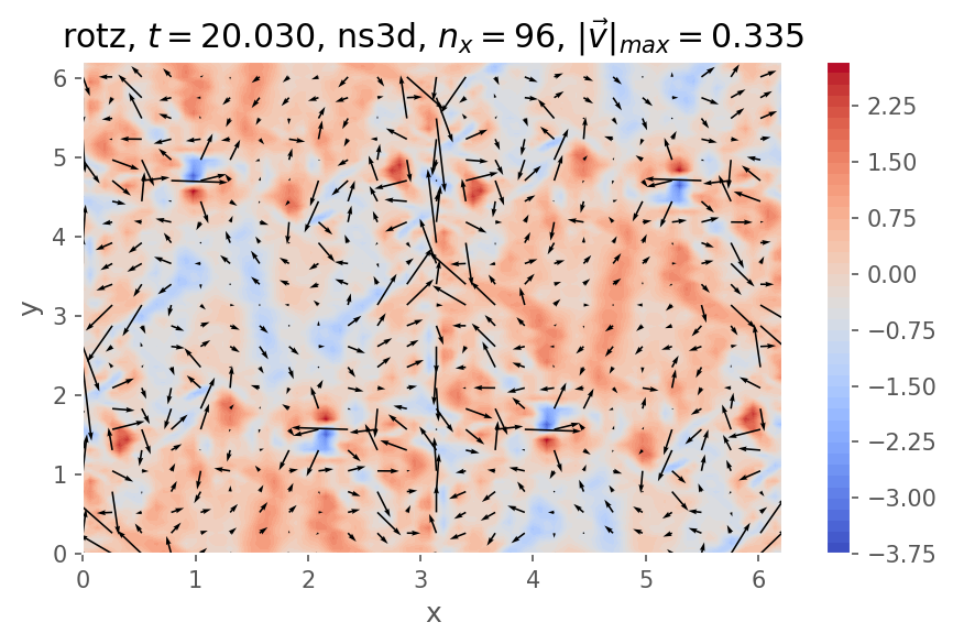
A cross-section of the z-component of vorticity
%matplotlib inline
plt.figure(0, dpi=150)
sim.output.phys_fields.plot(
    equation=f"x={sim.oper.Lx / 4}", numfig=0, nb_contours=50, cmap="coolwarm"
)
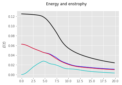
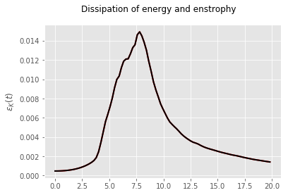
Spatially averaged energy, enstrophy and their dissipation rates
sim.output.spatial_means.plot()
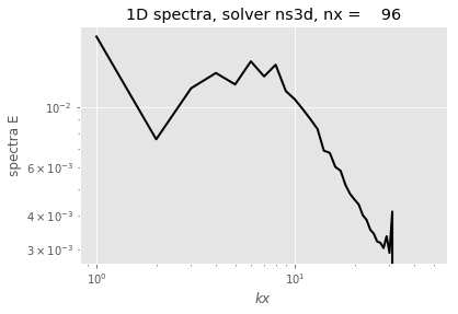
Compensated kinetic energy spectra
sim.output.spectra.plot1d(tmin=15, tmax=20, coef_compensate=5 / 3)
plot1d(tmin=15, tmax=20, delta_t=None, coef_compensate=1.667)
plot 1D spectra
    tmin =  14.8653 ; tmax =   19.627 ; delta_t = None
    imin =       29 ; imax =       38 ; delta_i = None