Part 2. Analyze one simulation
from pathlib import Path
%matplotlib inline
import matplotlib.pyplot as plt

plt.rc("figure", dpi=80)
import fluidsim as fls

path_dir_data = Path(fls.FLUIDSIM_PATH) / "tutorial_parametric_study"
path_runs = sorted(path_dir_data.glob("*"), key=lambda p: p.name)
[p.name for p in path_runs]
['ns3d.strat_144x144x48_V4.5x4.5x1.5_N0.2_Lf3.5_U0.01_D0.5_2021-10-05_15-35-47',
 'ns3d.strat_144x144x48_V4.5x4.5x1.5_N0.2_Lf3.5_U0.02_D0.5_2021-10-05_16-12-36',
 'ns3d.strat_144x144x48_V4.5x4.5x1.5_N0.2_Lf3.5_U0.04_D0.5_2021-10-05_16-49-31',
 'ns3d.strat_144x144x48_V4.5x4.5x1.5_N0.2_Lf3.5_U0.06_D0.5_2021-10-05_17-25-48',
 'ns3d.strat_144x144x48_V4.5x4.5x1.5_N0.2_Lf3.5_U0.08_D0.5_2021-10-05_18-01-23']
Let’s first recreate a sim object with the last directory:
from fluidsim import load
sim = load(path_runs[-3])
*************************************
Program fluidsim
sim:                <class 'fluidsim_core.extend_simul.extend_simul_class.<locals>.NewSimul'>
sim.output:         <class 'fluidsim.solvers.ns3d.strat.output.Output'>
sim.oper:           <class 'fluidsim.operators.operators3d.OperatorsPseudoSpectral3D'>
sim.state:          <class 'fluidsim.solvers.ns3d.strat.state.StateNS3DStrat'>
sim.time_stepping:  <class 'fluidsim.solvers.ns3d.time_stepping.TimeSteppingPseudoSpectralNS3D'>
sim.init_fields:    <class 'fluidsim.solvers.ns3d.init_fields.InitFieldsNS3D'>
sim.forcing:        <class 'fluidsim.solvers.ns3d.forcing.ForcingNS3D'>

solver ns3d.strat, RK4 and sequential,
type fft: fluidfft.fft3d.with_pyfftw
nx =      4 ; ny =      4 ; nz =      4
Lx = 4.5 ; Ly = 4.5 ; Lz = 1.5
path_run =
/home/pierre/Sim_data/tutorial_parametric_study/ns3d.strat_144x144x48_V4.5x4.5x1.5_N0.2_Lf3.5_U0.04_D0.5_2021-10-05_16-49-31
init_fields.type: constant

Initialization outputs:
sim.output.phys_fields:       <class 'fluidsim.base.output.phys_fields3d.PhysFieldsBase3D'>
sim.output.spatial_means:     <class 'fluidsim.solvers.ns3d.strat.output.spatial_means.SpatialMeansNS3DStrat'>
sim.output.spatial_means_regions:<class 'fluidsim.extend_simul.spatial_means_regions_milestone.SpatialMeansRegions'>
sim.output.spatiotemporal_spectra:<class 'fluidsim.solvers.ns3d.output.spatiotemporal_spectra.SpatioTemporalSpectraNS3D'>
sim.output.spectra:           <class 'fluidsim.solvers.ns3d.strat.output.spectra.SpectraNS3DStrat'>
sim.output.spect_energy_budg: <class 'fluidsim.solvers.ns3d.strat.output.spect_energy_budget.SpectralEnergyBudgetNS3DStrat'>
sim.output.temporal_spectra:  <class 'fluidsim.base.output.temporal_spectra.TemporalSpectra3D'>

Memory usage at the end of init. (equiv. seq.): 192.16015625 Mo
Size of state_spect (equiv. seq.): 0.003072 Mo
The object sim created from the simulation directory is very similar to the object sim used during the simulation. However, since it has been created with the function fluidsim.load (and not with fluidsim.load_for_restart), it is light (no state loaded and no operators created) and we cannot restart the simulation with this object. But we can easily get a lot of information on the simulation and of course, plot some figures!
Get the parameters of the simulation
sim.params.oper
<fluidsim_core.params.Parameters object at 0x7faf5ff92e50>

<oper Lx="4.5" Ly="4.5" Lz="1.5" NO_SHEAR_MODES="True" coef_dealiasing="0.8"
      nx="144" ny="144" nz="48" truncation_shape="cubic" type_fft="default"
      type_fft2d="sequential"/>
sim.params.forcing.type
'milestone'
sim.params.forcing.milestone
<fluidsim_core.params.Parameters object at 0x7faf5ff9ea30>

<milestone nx_max="48">
  <objects diameter="0.5" number="3" type="cylinders"
           width_boundary_layers="0.1"/>

  <movement type="periodic_uniform">
    <uniform speed="1.0"/>

    <sinusoidal length="1.0" period="1.0"/>

    <periodic_uniform length="3.5" length_acc="0.25" speed="0.04"/>

  </movement>

</milestone>
Which data were saved?
sim.output.path_run
'/home/pierre/Sim_data/tutorial_parametric_study/ns3d.strat_144x144x48_V4.5x4.5x1.5_N0.2_Lf3.5_U0.04_D0.5_2021-10-05_16-49-31'
!ls {sim.output.path_run}
info_solver.xml           state_phys_t00040.140.nc  state_phys_t00260.103.nc
params_simul.xml          state_phys_t00060.192.nc  state_phys_t00280.063.nc
spatial_means.txt         state_phys_t00080.095.nc  state_phys_t00300.130.nc
spatial_means_regions     state_phys_t00100.153.nc  state_phys_t00320.129.nc
spatiotemporal            state_phys_t00120.176.nc  state_phys_t00340.151.nc
spectra1d.h5              state_phys_t00140.150.nc  state_phys_t00360.094.nc
spectra3d.h5              state_phys_t00160.073.nc  state_phys_t00380.129.nc
spectra_kzkh.h5           state_phys_t00180.065.nc  state_phys_t00400.025.nc
spect_energy_budg.h5      state_phys_t00200.093.nc  stdout.txt
state_phys_t00000.000.nc  state_phys_t00220.007.nc
state_phys_t00020.268.nc  state_phys_t00240.006.nc
!ls {sim.output.path_run + "/spatiotemporal"}
rank00000_tmin00000.000.h5 rank00001_tmin00000.000.h5
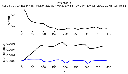
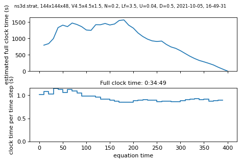
Representation of the information printed in the log
sim.output.print_stdout.plot()
sim.output.print_stdout.plot_clock_times()
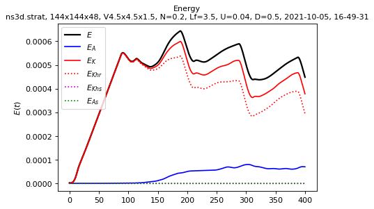
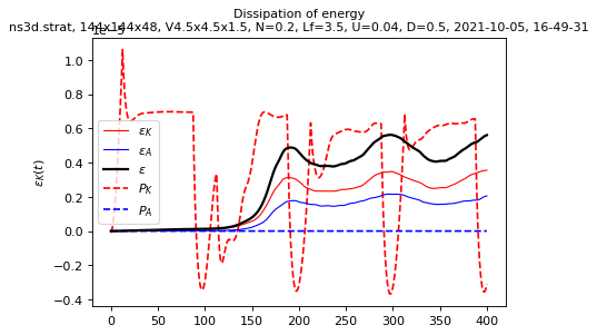
Spatial means saved in spatial_means.txt
sim.output.spatial_means.plot()
info_forcing = sim.forcing.get_info()
info_forcing
{'period': 200.0}
period = info_forcing["period"]
?sim.output.spatial_means.get_dimless_numbers_averaged
Signature: sim.output.spatial_means.get_dimless_numbers_averaged(tmin=0, tmax=None)
Docstring: <no docstring>
File:      ~/Dev/fluidsim/fluidsim/solvers/ns3d/strat/output/spatial_means.py
Type:      method
dimless_numbers = sim.output.spatial_means.get_dimless_numbers_averaged(
    tmin=period
)
dimless_numbers
{'Fh': 0.03442003363915731,
 'R2': 70.8592505,
 'R4': 30.29826938649225,
 'epsK2/epsK': 0.042376597274872044,
 'Gamma': 0.6186840670881376,
 'dimensional': {'Uh2': 0.0004185852799, 'epsK': 2.83437002e-06}}
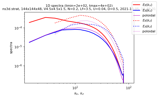
Spectra saved in spectra1d.h5
?sim.output.spectra.plot1d
Signature:
sim.output.spectra.plot1d(
    tmin=0,
    tmax=None,
    coef_compensate=0,
    coef_plot_k3=None,
    coef_plot_k53=None,
    coef_plot_k2=None,
    xlim=None,
    ylim=None,
    directions=('x', 'z'),
)
Docstring: <no docstring>
File:      ~/Dev/fluidsim/fluidsim/solvers/ns3d/output/spectra.py
Type:      method
sim.output.spectra.plot1d(tmin=period, coef_compensate=5 / 3)
plot1d(tmin=     200, tmax= 400.025, coef_compensate=1.667)
plot 1D spectra
tmin =  200.093 ; tmax =  400.025
imin =      100 ; imax =      200
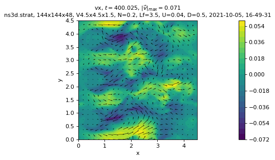
Simple cross-sections of the flow fields
sim.output.phys_fields.plot()
?sim.output.phys_fields.plot
Signature:
sim.output.phys_fields.plot(
    field=None,
    time=None,
    QUIVER=True,
    vector='v',
    equation=None,
    nb_contours=20,
    type_plot='contourf',
    vmin=None,
    vmax=None,
    cmap=None,
    numfig=None,
    SCALED=True,
)
Docstring:
Plot a field.

Parameters
----------

field : {str, np.ndarray}, optional

time : number, optional

QUIVER : True

vecx : 'ux'

vecy : 'uy'

nb_contours : 20

type_plot : 'contourf'

vmin : None

vmax : None

cmap : None (usually 'viridis')

numfig : None
File:      ~/Dev/fluidsim/fluidsim/base/output/phys_fields3d.py
Type:      method
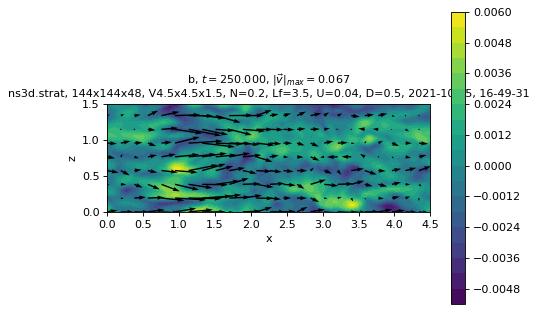
sim.output.phys_fields.plot(
    field="b", time=1.25 * period, equation=f"y={sim.params.oper.Lx / 2}"
)
?sim.output.phys_fields.animate
Signature:
sim.output.phys_fields.animate(
    key_field=None,
    dt_frame_in_sec=0.3,
    dt_equations=None,
    tmin=None,
    tmax=None,
    repeat=True,
    save_file=False,
    numfig=None,
    fargs={},
    fig_kw={},
    **kwargs,
)
Docstring:
Load the key field from multiple save files and display as
an animated plot or save as a movie file.

Parameters
----------
key_field : str
    Specifies which field to animate
dt_frame_in_sec : float
    Interval between animated frames in seconds
dt_equations : float
    Approx. interval between saved files to load in simulation time
    units
tmax : float
    Animate till time `tmax`.
repeat : bool
    Loop the animation
save_file : str or bool
    Path to save the movie. When `True`  saves into a file instead
    of plotting it on screen (default: ~/fluidsim_movie.mp4). Specify
    a string to save to another file location. Format is autodetected
    from the filename extension.
numfig : int
    Figure number on the window
fargs : dict
    Dictionary of arguments for `update_animation`. Matplotlib
    requirement.
fig_kw : dict
    Dictionary of arguments for arguments for the figure.

Other Parameters
----------------
All `kwargs` are passed on to `init_animation` and `_ani_save`

xmax : float
    Set x-axis limit for 1D animated plots
ymax : float
    Set y-axis limit for 1D animated plots
clim : tuple
    Set colorbar limits for 2D animated plots
step : int
    Set step value to get a coarse 2D field
QUIVER : bool
    Set quiver on or off on top of 2D pcolor plots
codec : str
    Codec used to save into a movie file (default: ffmpeg)

Examples
--------
>>> import fluidsim as fls
>>> sim = fls.load_sim_for_plot()
>>> animate = sim.output.spectra.animate
>>> animate('E')
>>> animate('rot')
>>> animate('rot', dt_equations=0.1, dt_frame_in_sec=50, clim=(-5, 5))
>>> animate('rot', clim=(-300, 300), fig_kw={"figsize": (14, 4)})
>>> animate('rot', tmax=25, clim=(-5, 5), save_file='True')
>>> animate('rot', clim=(-5, 5), save_file='~/fluidsim.gif', codec='imagemagick')

.. TODO: Use FuncAnimation with blit=True option.

Notes
-----

This method is kept as generic as possible. Any arguments specific to
1D, 2D or 3D animations or specific to a type of output are be passed
via keyword arguments (``kwargs``) into its respective
``init_animation`` or ``update_animation`` methods.
File:      ~/Dev/fluidsim/fluidsim/base/output/movies.py
Type:      method
How to use Paraview or Visit?
For serious 3D representations, it is easy to use specialized software like Paraview or Visit. These programs are able to open .xmf files which describe how the physical fields are stored in the hdf5 / netcdf fluidsim files.
One needs to create the .xmf file with the command line tool fluidsim-create-xml-description.
! fluidsim-create-xml-description {sim.output.path_run}
Creation of the file /home/pierre/Sim_data/tutorial_parametric_study/ns3d.strat_144x144x48_V4.5x4.5x1.5_N0.2_Lf3.5_U0.04_D0.5_2021-10-05_16-49-31/states_phys.xmf
Open it with a Xdmf reader to read the output files.
! ls {sim.output.path_run + "/*.xmf"}
/home/pierre/Sim_data/tutorial_parametric_study/ns3d.strat_144x144x48_V4.5x4.5x1.5_N0.2_Lf3.5_U0.04_D0.5_2021-10-05_16-49-31/states_phys.xmf
!head -20 {sim.output.path_run + "/states_phys.xmf"}
<?xml version="1.0" ?>
<!DOCTYPE Xdmf SYSTEM "Xdmf.dtd" []>
<Xdmf>
  <Domain>
    <Grid Name="TimeSeries" GridType="Collection"
          CollectionType="Temporal">

    <Grid Name="my_uniform_grid" GridType="Uniform">
      <Time Value="0.000000000" />
      <Topology TopologyType="3DCoRectMesh" Dimensions="48 144 144">
      </Topology>
      <Geometry GeometryType="Origin_DxDyDz">
        <DataItem Dimensions="3" NumberType="Float" Format="XML">
        0 0 0
        </DataItem>
        <DataItem Dimensions="3" NumberType="Float" Format="XML">
        0.03125 0.03125 0.03125
        </DataItem>
      </Geometry>
Spatiotemporal spectra
?sim.output.spatiotemporal_spectra.plot_temporal_spectra
Signature:
sim.output.spatiotemporal_spectra.plot_temporal_spectra(
    key_field=None,
    tmin=0,
    tmax=None,
    dtype=None,
    xscale='log',
)
Docstring: plot the temporal spectra computed from the 4d spectra
File:      ~/Dev/fluidsim/fluidsim/base/output/spatiotemporal_spectra.py
Type:      method
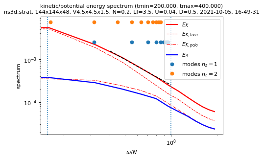
sim.output.spatiotemporal_spectra.plot_temporal_spectra(tmin=period)
load times series...
tmin= 204.215, tmax= 392.828, nit=25
performing time fft...
load times series...
tmin= 204.215, tmax= 392.828, nit=25
computing temporal spectra...
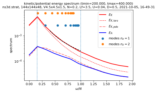
sim.output.spatiotemporal_spectra.plot_temporal_spectra(
    tmin=period, xscale="linear"
)
?sim.output.spatiotemporal_spectra.plot_kzkhomega
Signature:
sim.output.spatiotemporal_spectra.plot_kzkhomega(
    key_field=None,
    tmin=0,
    tmax=None,
    dtype=None,
    equation=None,
    xmax=None,
    ymax=None,
    cmap=None,
    vmin=None,
    vmax=None,
)
Docstring:
plot the spatiotemporal spectra, with a cylindrical average in k-space

equation must start with 'omega=', 'kh=', 'kz=', 'ikh=' or 'ikz='.
File:      ~/Dev/fluidsim/fluidsim/base/output/spatiotemporal_spectra.py
Type:      method
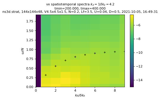
sim.output.spatiotemporal_spectra.plot_kzkhomega(tmin=period, equation="ikz=1")
Computing spectra...
load times series...
tmin= 204.215, tmax= 392.828, nit=25
performing time fft...
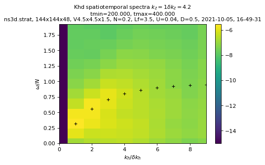
sim.output.spatiotemporal_spectra.plot_kzkhomega(
    key_field="Khd", tmin=period, equation="ikz=1"
)
Computing spectra...
load times series...
tmin= 204.215, tmax= 392.828, nit=25
performing time fft...
Computing ur, ud spectra...
load times series...
tmin= 204.215, tmax= 392.828, nit=25
computing temporal spectra...