Restart and resolution change
Fluidsim provides 2 command-line tools to restart a simulation (fluidsim-restart)
and create a new file with a modified resolution (fluidsim-modif-resolution).
Let’s present these very useful tools!
First, one can get help by invoking these tools with the -h option:
!fluidsim-restart -h
usage: fluidsim-restart [-h] [-oc] [-oi] [--modify-params MODIFY_PARAMS]
                        [--new-dir-results] [--t_approx T_APPROX]
                        [--add-to-t_end ADD_TO_T_END]
                        [--add-to-it_end ADD_TO_IT_END] [--t_end T_END]
                        [--it_end IT_END] [--merge-missing-params]
                        [--max-elapsed MAX_ELAPSED]
                        path

Restart a fluidsim simulation

positional arguments:
  path                  Path of the directory or file from which to restart

options:
  -h, --help            show this help message and exit
  -oc, --only-check     Only check what should be done
  -oi, --only-init      Only run initialization phase
  --modify-params MODIFY_PARAMS
                        Code modifying the `params` object.
  --new-dir-results     Create a new directory for the new simulation
  --t_approx T_APPROX   Approximate time to choose the file from which to
                        restart
  --add-to-t_end ADD_TO_T_END
                        Time added to params.time_stepping.t_end
  --add-to-it_end ADD_TO_IT_END
                        Number of steps added to params.time_stepping.it_end
  --t_end T_END         params.time_stepping.t_end
  --it_end IT_END       params.time_stepping.it_end
  --merge-missing-params
                        Can be used to load old simulations carried out with
                        an old fluidsim version.
  --max-elapsed MAX_ELAPSED
                        Maximum elapsed time.
!fluidsim-modif-resolution -h
usage: fluidsim-modif-resolution [-h] [--t_approx T_APPROX]
                                 path coef_modif_resol

Create a new state file with a different resolution

positional arguments:
  path                 Input: path towards a directory or a file
  coef_modif_resol     Input: coefficient of resolution change

options:
  -h, --help           show this help message and exit
  --t_approx T_APPROX  Approximate time to choose the file from which to
                       restart
Then, let’s use these tools. First we need a simulation directory.
from fluidsim.util.scripts.turb_trandom_anisotropic import main

params, sim = main(
    args=(
        '--sub-directory "doc_aniso" -nz 12 --ratio-nh-nz 2 --t_end 1 '
        '--modify-params "params.output.periods_print.print_stdout = 0.25; '
        'params.output.periods_save.spect_energy_budg = 0"'
    )
)
Namespace(only_print_params_as_code=False, only_print_params=False, only_plot_forcing=False, nz=12, ratio_nh_nz=2, t_end=1.0, N=10.0, nu=None, nu4=None, Rb=None, Rb4=None, coef_nu4=1.0, forced_field='polo', init_velo_max=0.01, nh_forcing=3, ratio_kfmin_kf=0.5, ratio_kfmax_kf=2.0, F=0.3, delta_F=0.1, spatiotemporal_spectra=False, projection=None, disable_no_vz_kz0=False, disable_NO_SHEAR_MODES=False, max_elapsed='23:50:00', coef_dealiasing=0.8, periods_save_phys_fields=1.0, sub_directory='doc_aniso', modify_params='params.output.periods_print.print_stdout = 0.25; params.output.periods_save.spect_energy_budg = 0')
Input horizontal Froude number: 0.1
eta * k_max = 1.902e-01
Resolution too coarse, we add order-4 hyper viscosity nu_4=4.524e-05.
angle = 17.46°
params.forcing.nkmin_forcing = 2.5
params.forcing.nkmax_forcing = 6
*************************************
Program fluidsim
sim:                <class 'fluidsim.solvers.ns3d.strat.solver.Simul'>
sim.output:         <class 'fluidsim.solvers.ns3d.strat.output.Output'>
sim.oper:           <class 'fluidsim.operators.operators3d.OperatorsPseudoSpectral3D'>
sim.state:          <class 'fluidsim.solvers.ns3d.strat.state.StateNS3DStrat'>
sim.time_stepping:  <class 'fluidsim.solvers.ns3d.time_stepping.TimeSteppingPseudoSpectralNS3D'>
sim.init_fields:    <class 'fluidsim.solvers.ns3d.init_fields.InitFieldsNS3D'>
sim.forcing:        <class 'fluidsim.solvers.ns3d.forcing.ForcingNS3D'>

solver ns3d.strat, RK4 and sequential,
type fft: fluidfft.fft3d.with_pyfftw
nx =     24 ; ny =     24 ; nz =     12
Lx = 3 ; Ly = 3 ; Lz = 1.5
path_run =
/tmp/sim_data/doc_aniso/ns3d.strat_polo_Fh1.000e-01_24x24x12_V3x3x1.5_fNone_N10_2025-12-03_21-57-43
init_fields.type: noise

To plot the forcing modes, you can use:
sim.forcing.forcing_maker.plot_forcing_region()

Initialization outputs:
sim.output.cross_corr:             <class 'fluidsim.base.output.cross_corr3d.CrossCorrelations'>
sim.output.phys_fields:            <class 'fluidsim.base.output.phys_fields3d.PhysFieldsBase3D'>
sim.output.spatial_means:          <class 'fluidsim.solvers.ns3d.strat.output.spatial_means.SpatialMeansNS3DStrat'>
sim.output.spatiotemporal_spectra: <class 'fluidsim.solvers.ns3d.output.spatiotemporal_spectra.SpatioTemporalSpectraNS3D'>
sim.output.spectra:                <class 'fluidsim.solvers.ns3d.strat.output.spectra.SpectraNS3DStrat'>
sim.output.spect_energy_budg:      <class 'fluidsim.solvers.ns3d.strat.output.spect_energy_budget.SpectralEnergyBudgetNS3DStrat'>
sim.output.temporal_spectra:       <class 'fluidsim.base.output.temporal_spectra.TemporalSpectra3D'>

Memory usage at the end of init. (equiv. seq.): 242.109375 Mo
Size of state_spect (equiv. seq.): 0.239616 Mo
*************************************
Beginning of the computation
save state_phys in file state_phys_t000.000.nc
    compute until t =          1
it =      0 ; t =            0 ; deltat  =    0.03927
              energy = 8.258e-06 ; Delta energy = +0.000e+00
MEMORY_USAGE:                  242.734375 Mo
it =      7 ; t =     0.274889 ; deltat  =    0.03927
              energy = 7.868e-02 ; Delta energy = +7.867e-02
              estimated remaining duration = 0:00:03
MEMORY_USAGE:                  244.109375 Mo
it =     13 ; t =     0.510509 ; deltat  =    0.03927
              energy = 9.740e-02 ; Delta energy = +1.872e-02
              estimated remaining duration = 0:00:02
MEMORY_USAGE:                  244.234375 Mo
it =     20 ; t =     0.785398 ; deltat  =    0.03927
              energy = 1.037e-01 ; Delta energy = +6.248e-03
              estimated remaining duration = 0:00:01
MEMORY_USAGE:                  244.234375 Mo
it =     26 ; t =      1.02102 ; deltat  =    0.03927
              energy = 1.070e-01 ; Delta energy = +3.327e-03
MEMORY_USAGE:                  244.359375 Mo
save state_phys in file state_phys_t001.021.nc
Computation completed in  4.24694 s
path_run =
/tmp/sim_data/doc_aniso/ns3d.strat_polo_Fh1.000e-01_24x24x12_V3x3x1.5_fNone_N10_2025-12-03_21-57-43

# To visualize the output with Paraview, create a file states_phys.xmf with:

fluidsim-create-xml-description /tmp/sim_data/doc_aniso/ns3d.strat_polo_Fh1.000e-01_24x24x12_V3x3x1.5_fNone_N10_2025-12-03_21-57-43

# To visualize with fluidsim:

fluidsim-ipy-load /tmp/sim_data/doc_aniso/ns3d.strat_polo_Fh1.000e-01_24x24x12_V3x3x1.5_fNone_N10_2025-12-03_21-57-43

# in IPython:

sim.output.phys_fields.set_equation_crosssection('x=1.5')
sim.output.phys_fields.animate('b')
We then define a variable with the path of the directory containing the results of the simulation.
sim.output.path_run
'/tmp/sim_data/doc_aniso/ns3d.strat_polo_Fh1.000e-01_24x24x12_V3x3x1.5_fNone_N10_2025-12-03_21-57-43'
from pprint import pprint


def ls_path_run(glob="*"):
    pprint(sorted(p.name for p in Path(sim.output.path_run).glob(glob)))


ls_path_run()
['coarse-oper-info.txt',
 'cross_corr1d.h5',
 'cross_corr3d.h5',
 'cross_corr_kzkh.h5',
 'info_solver.xml',
 'params_simul.xml',
 'spatial_means.txt',
 'spectra1d.h5',
 'spectra3d.h5',
 'spectra_kzkh.h5',
 'state_phys_t000.000.nc',
 'state_phys_t001.021.nc',
 'stdout.txt']
sim.output.spatial_means.plot()
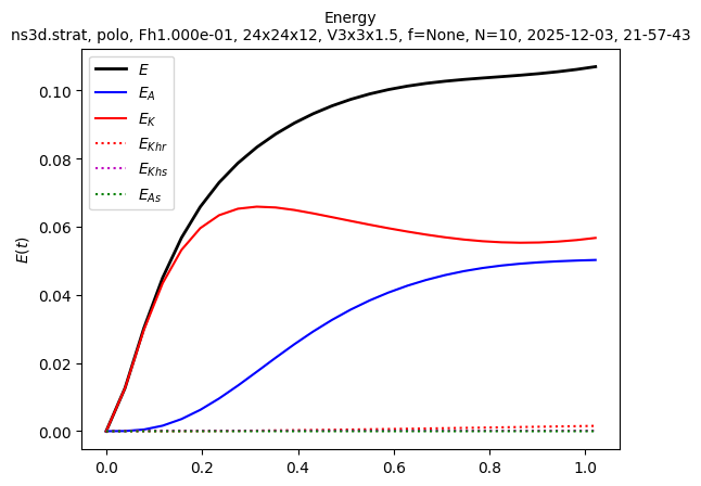
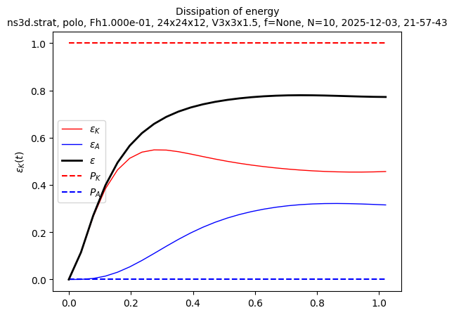
Ah, we see that t_end = 1 was not enough to obtain a statistically steady state. We need to run the simulation longer. Let’s restart it to run until t_end = 2:
!fluidsim-restart {sim.output.path_run} --t_end 2.0
Namespace(path='/tmp/sim_data/doc_aniso/ns3d.strat_polo_Fh1.000e-01_24x24x12_V3x3x1.5_fNone_N10_2025-12-03_21-57-43', only_check=False, only_init=False, modify_params=None, new_dir_results=False, t_approx=None, add_to_t_end=None, add_to_it_end=None, t_end=2.0, it_end=None, merge_missing_params=False, max_elapsed=None)
/home/docs/checkouts/readthedocs.org/user_builds/fluidsim/envs/stable/lib/python3.11/site-packages/fluidsim/operators/operators2d.py:36: UserWarning: operators2d.py has to be pythranized to be efficient! Install pythran and recompile.
  warn(
/tmp/sim_data/doc_aniso/ns3d.strat_polo_Fh1.000e-01_24x24x12_V3x3x1.5_fNone_N10_2025-12-03_21-57-43/state_phys_t001.021.nc
*************************************
Program fluidsim
sim:                <class 'fluidsim.solvers.ns3d.strat.solver.Simul'>
sim.output:         <class 'fluidsim.solvers.ns3d.strat.output.Output'>
sim.oper:           <class 'fluidsim.operators.operators3d.OperatorsPseudoSpectral3D'>
sim.state:          <class 'fluidsim.solvers.ns3d.strat.state.StateNS3DStrat'>
sim.time_stepping:  <class 'fluidsim.solvers.ns3d.time_stepping.TimeSteppingPseudoSpectralNS3D'>
sim.init_fields:    <class 'fluidsim.solvers.ns3d.init_fields.InitFieldsNS3D'>
sim.forcing:        <class 'fluidsim.solvers.ns3d.forcing.ForcingNS3D'>

solver ns3d.strat, RK4 and sequential,
type fft: fluidfft.fft3d.with_pyfftw
nx =     24 ; ny =     24 ; nz =     12
Lx = 3 ; Ly = 3 ; Lz = 1.5
path_run =
/tmp/sim_data/doc_aniso/ns3d.strat_polo_Fh1.000e-01_24x24x12_V3x3x1.5_fNone_N10_2025-12-03_21-57-43
init_fields.type: from_file

Load state from file:
[...]at_polo_Fh1.000e-01_24x24x12_V3x3x1.5_fNone_N10_2025-12-03_21-57-43/state_phys_t001.021.nc

To plot the forcing modes, you can use:
sim.forcing.forcing_maker.plot_forcing_region()

Initialization outputs:
sim.output.cross_corr:             <class 'fluidsim.base.output.cross_corr3d.CrossCorrelations'>
sim.output.phys_fields:            <class 'fluidsim.base.output.phys_fields3d.PhysFieldsBase3D'>
sim.output.spatial_means:          <class 'fluidsim.solvers.ns3d.strat.output.spatial_means.SpatialMeansNS3DStrat'>
sim.output.spatiotemporal_spectra: <class 'fluidsim.solvers.ns3d.output.spatiotemporal_spectra.SpatioTemporalSpectraNS3D'>
sim.output.spectra:                <class 'fluidsim.solvers.ns3d.strat.output.spectra.SpectraNS3DStrat'>
sim.output.spect_energy_budg:      <class 'fluidsim.solvers.ns3d.strat.output.spect_energy_budget.SpectralEnergyBudgetNS3DStrat'>
sim.output.temporal_spectra:       <class 'fluidsim.base.output.temporal_spectra.TemporalSpectra3D'>

Memory usage at the end of init. (equiv. seq.): 226.13671875 Mo
Size of state_spect (equiv. seq.): 0.239616 Mo
*************************************
Beginning of the computation
    compute until t =          2
it =     26 ; t =      1.02102 ; deltat  =    0.03927
              energy = 1.070e-01 ; Delta energy = +0.000e+00

MEMORY_USAGE:                  226.13671875 Mo
it =     32 ; t =      1.25664 ; deltat  =    0.03927
              energy = 1.141e-01 ; Delta energy = +7.157e-03
              estimated remaining duration = 0:00:03
MEMORY_USAGE:                  227.88671875 Mo
it =     39 ; t =      1.53153 ; deltat  =    0.03927
              energy = 1.224e-01 ; Delta energy = +8.255e-03
              estimated remaining duration = 0:00:02
MEMORY_USAGE:                  228.13671875 Mo
it =     45 ; t =      1.76715 ; deltat  =    0.03927
              energy = 1.250e-01 ; Delta energy = +2.609e-03
              estimated remaining duration = 0:00:01
MEMORY_USAGE:                  228.26171875 Mo
it =     51 ; t =      2.00277 ; deltat  =    0.03927
              energy = 1.240e-01 ; Delta energy = -9.659e-04

MEMORY_USAGE:                  228.38671875 Mo
save state_phys in file state_phys_t002.003.nc
Computation completed in    4.059 s
path_run =
/tmp/sim_data/doc_aniso/ns3d.strat_polo_Fh1.000e-01_24x24x12_V3x3x1.5_fNone_N10_2025-12-03_21-57-43

# To visualize with IPython:

fluidsim-ipy-load /tmp/sim_data/doc_aniso/ns3d.strat_polo_Fh1.000e-01_24x24x12_V3x3x1.5_fNone_N10_2025-12-03_21-57-43
ls_path_run()
['coarse-oper-info.txt',
 'cross_corr1d.h5',
 'cross_corr3d.h5',
 'cross_corr_kzkh.h5',
 'info_solver.xml',
 'params_simul.xml',
 'spatial_means.txt',
 'spectra1d.h5',
 'spectra3d.h5',
 'spectra_kzkh.h5',
 'state_phys_t000.000.nc',
 'state_phys_t001.021.nc',
 'state_phys_t002.003.nc',
 'stdout.txt']
sim.output.spatial_means.plot()
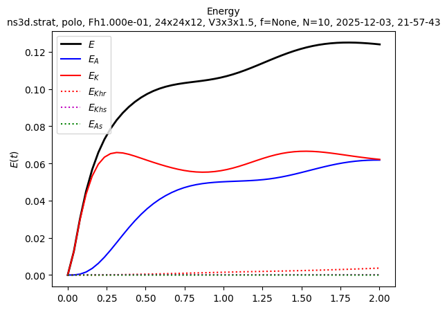
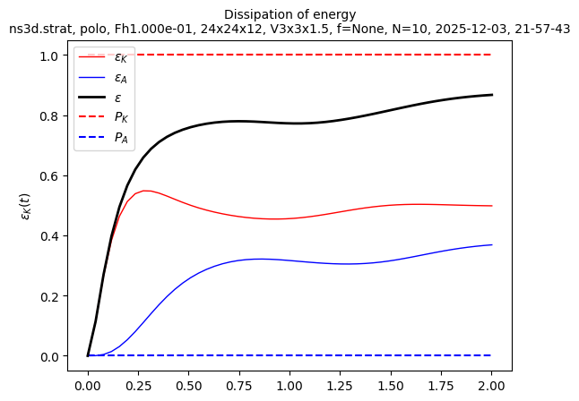
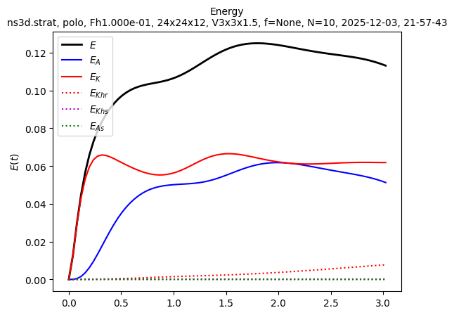
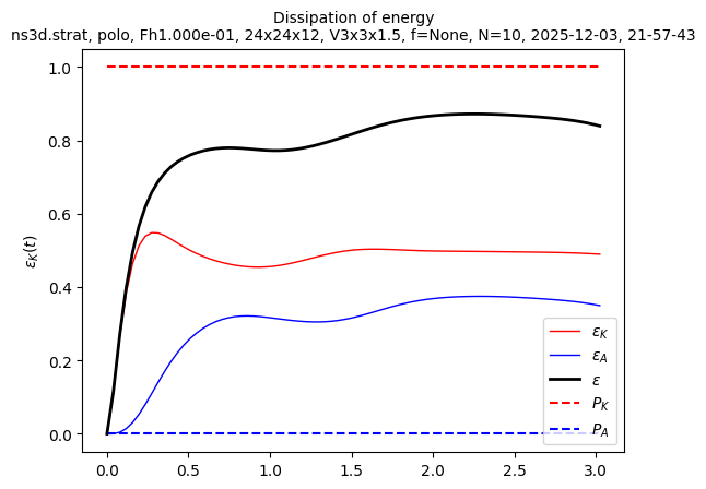
Finally, we are not far from a statistically steady state. We can relaunch the simulation to save results about this state. Here we show how to restart a simulation with the spatiotemporal spectra output activated:
!fluidsim-restart {sim.output.path_run} --t_end 3.0 --modify-params "params.output.periods_save.spatiotemporal_spectra = 2 * pi / (4 * params.N)"
Namespace(path='/tmp/sim_data/doc_aniso/ns3d.strat_polo_Fh1.000e-01_24x24x12_V3x3x1.5_fNone_N10_2025-12-03_21-57-43', only_check=False, only_init=False, modify_params='params.output.periods_save.spatiotemporal_spectra = 2 * pi / (4 * params.N)', new_dir_results=False, t_approx=None, add_to_t_end=None, add_to_it_end=None, t_end=3.0, it_end=None, merge_missing_params=False, max_elapsed=None)
/home/docs/checkouts/readthedocs.org/user_builds/fluidsim/envs/stable/lib/python3.11/site-packages/fluidsim/operators/operators2d.py:36: UserWarning: operators2d.py has to be pythranized to be efficient! Install pythran and recompile.
  warn(
/tmp/sim_data/doc_aniso/ns3d.strat_polo_Fh1.000e-01_24x24x12_V3x3x1.5_fNone_N10_2025-12-03_21-57-43/state_phys_t002.003.nc
*************************************
Program fluidsim
sim:                <class 'fluidsim.solvers.ns3d.strat.solver.Simul'>
sim.output:         <class 'fluidsim.solvers.ns3d.strat.output.Output'>
sim.oper:           <class 'fluidsim.operators.operators3d.OperatorsPseudoSpectral3D'>
sim.state:          <class 'fluidsim.solvers.ns3d.strat.state.StateNS3DStrat'>
sim.time_stepping:  <class 'fluidsim.solvers.ns3d.time_stepping.TimeSteppingPseudoSpectralNS3D'>
sim.init_fields:    <class 'fluidsim.solvers.ns3d.init_fields.InitFieldsNS3D'>
sim.forcing:        <class 'fluidsim.solvers.ns3d.forcing.ForcingNS3D'>

solver ns3d.strat, RK4 and sequential,
type fft: fluidfft.fft3d.with_pyfftw
nx =     24 ; ny =     24 ; nz =     12
Lx = 3 ; Ly = 3 ; Lz = 1.5
path_run =
/tmp/sim_data/doc_aniso/ns3d.strat_polo_Fh1.000e-01_24x24x12_V3x3x1.5_fNone_N10_2025-12-03_21-57-43
init_fields.type: from_file

Load state from file:
[...]at_polo_Fh1.000e-01_24x24x12_V3x3x1.5_fNone_N10_2025-12-03_21-57-43/state_phys_t002.003.nc

To plot the forcing modes, you can use:
sim.forcing.forcing_maker.plot_forcing_region()

Initialization outputs:
sim.output.cross_corr:             <class 'fluidsim.base.output.cross_corr3d.CrossCorrelations'>
sim.output.phys_fields:            <class 'fluidsim.base.output.phys_fields3d.PhysFieldsBase3D'>
sim.output.spatial_means:          <class 'fluidsim.solvers.ns3d.strat.output.spatial_means.SpatialMeansNS3DStrat'>
sim.output.spatiotemporal_spectra: <class 'fluidsim.solvers.ns3d.output.spatiotemporal_spectra.SpatioTemporalSpectraNS3D'>
sim.output.spectra:                <class 'fluidsim.solvers.ns3d.strat.output.spectra.SpectraNS3DStrat'>
sim.output.spect_energy_budg:      <class 'fluidsim.solvers.ns3d.strat.output.spect_energy_budget.SpectralEnergyBudgetNS3DStrat'>
sim.output.temporal_spectra:       <class 'fluidsim.base.output.temporal_spectra.TemporalSpectra3D'>

Memory usage at the end of init. (equiv. seq.): 226.7578125 Mo
Size of state_spect (equiv. seq.): 0.239616 Mo
*************************************
Beginning of the computation
    compute until t =          3
it =     51 ; t =      2.00277 ; deltat  =    0.03927
              energy = 1.240e-01 ; Delta energy = +0.000e+00

MEMORY_USAGE:                  226.7578125 Mo
it =     58 ; t =      2.27765 ; deltat  =    0.03927
              energy = 1.213e-01 ; Delta energy = -2.778e-03
              estimated remaining duration = 0:00:03
MEMORY_USAGE:                  228.3828125 Mo
it =     64 ; t =      2.51327 ; deltat  =    0.03927
              energy = 1.192e-01 ; Delta energy = -2.034e-03
              estimated remaining duration = 0:00:02
MEMORY_USAGE:                  228.5078125 Mo
it =     71 ; t =      2.78816 ; deltat  =    0.03927
              energy = 1.169e-01 ; Delta energy = -2.298e-03
              estimated remaining duration = 0:00:01
MEMORY_USAGE:                  228.6328125 Mo
it =     77 ; t =      3.02378 ; deltat  =    0.03927
              energy = 1.132e-01 ; Delta energy = -3.748e-03

MEMORY_USAGE:                  228.7578125 Mo
save state_phys in file state_phys_t003.024.nc
Computation completed in  4.24536 s
path_run =
/tmp/sim_data/doc_aniso/ns3d.strat_polo_Fh1.000e-01_24x24x12_V3x3x1.5_fNone_N10_2025-12-03_21-57-43

# To visualize with IPython:

fluidsim-ipy-load /tmp/sim_data/doc_aniso/ns3d.strat_polo_Fh1.000e-01_24x24x12_V3x3x1.5_fNone_N10_2025-12-03_21-57-43
ls_path_run()
['coarse-oper-info.txt',
 'cross_corr1d.h5',
 'cross_corr3d.h5',
 'cross_corr_kzkh.h5',
 'info_solver.xml',
 'params_simul.xml',
 'spatial_means.txt',
 'spatiotemporal',
 'spectra1d.h5',
 'spectra3d.h5',
 'spectra_kzkh.h5',
 'state_phys_t000.000.nc',
 'state_phys_t001.021.nc',
 'state_phys_t002.003.nc',
 'state_phys_t003.024.nc',
 'stdout.txt']
spatiotemporal is a directory containing the data that can be used to compute spatiotemporal spectra:
ls_path_run("spatiotemporal/*")
['rank00000_tmin002.003.h5']
sim.output.spatial_means.plot()
We want to start a larger simulation from the last state of this small simulation. We first need to create a larger file:
!fluidsim-modif-resolution {sim.output.path_run} 5/4
Namespace(path='/tmp/sim_data/doc_aniso/ns3d.strat_polo_Fh1.000e-01_24x24x12_V3x3x1.5_fNone_N10_2025-12-03_21-57-43', coef_modif_resol='5/4', t_approx=None)
Changing resolution of the state contained in
/tmp/sim_data/doc_aniso/ns3d.strat_polo_Fh1.000e-01_24x24x12_V3x3x1.5_fNone_N10_2025-12-03_21-57-43/state_phys_t003.024.nc
/home/docs/checkouts/readthedocs.org/user_builds/fluidsim/envs/stable/lib/python3.11/site-packages/fluidsim/operators/operators2d.py:36: UserWarning: operators2d.py has to be pythranized to be efficient! Install pythran and recompile.
  warn(
Memory usage after init operator "input":    0.185 Go
Memory usage after init operator "output":   0.185 Go
Memory usage after init fields:              0.185 Go
size field2:                                 0.000 Go
Memory usage after init field2:              0.185 Go
size field2_spect:                           0.000 Go
Memory usage after init field2_spect:        0.185 Go
Saving file state_phys_t003.024.nc...
get_var("vx")
- reading field from disk...    done in 0:00:00.005481
- forward fft smaller field...  done in 0:00:00.000067
- filling field2_fft...         done in 0:00:00.001015
- backward fft field2...        done in 0:00:00.000117
get_var("vy")
- reading field from disk...    done in 0:00:00.004665
- forward fft smaller field...  done in 0:00:00.000057
- filling field2_fft...         done in 0:00:00.000992
- backward fft field2...        done in 0:00:00.000086
get_var("vz")
- reading field from disk...    done in 0:00:00.004702
- forward fft smaller field...  done in 0:00:00.000056
- filling field2_fft...
done in 0:00:00.001575
- backward fft field2...        done in 0:00:00.000084
get_var("b")
- reading field from disk...    done in 0:00:00.004659
- forward fft smaller field...  done in 0:00:00.000056
- filling field2_fft...         done in 0:00:00.000988
- backward fft field2...        done in 0:00:00.000071
File state_phys_t003.024.nc saved in:
/tmp/sim_data/doc_aniso/ns3d.strat_polo_Fh1.000e-01_24x24x12_V3x3x1.5_fNone_N10_2025-12-03_21-57-43/State_phys_30x30x15
total duration: 0:00:01.063381
We can now launch the last simulation from the file just created.
path_new_state = next(Path(sim.output.path_run).glob("State_phys*"))
str(path_new_state)
'/tmp/sim_data/doc_aniso/ns3d.strat_polo_Fh1.000e-01_24x24x12_V3x3x1.5_fNone_N10_2025-12-03_21-57-43/State_phys_30x30x15'
!fluidsim-restart {path_new_state} --t_end 3.1 --modify-params "params.NEW_DIR_RESULTS = True; params.nu_2 /= 2; params.output.periods_print.print_stdout = 0.05; params.output.periods_save.spatial_means = 0.01;"
Namespace(path='/tmp/sim_data/doc_aniso/ns3d.strat_polo_Fh1.000e-01_24x24x12_V3x3x1.5_fNone_N10_2025-12-03_21-57-43/State_phys_30x30x15', only_check=False, only_init=False, modify_params='params.NEW_DIR_RESULTS = True; params.nu_2 /= 2; params.output.periods_print.print_stdout = 0.05; params.output.periods_save.spatial_means = 0.01;', new_dir_results=False, t_approx=None, add_to_t_end=None, add_to_it_end=None, t_end=3.1, it_end=None, merge_missing_params=False, max_elapsed=None)
load params from file
[...]1.000e-01_24x24x12_V3x3x1.5_fNone_N10_2025-12-03_21-57-43/State_phys_30x30x15/state_phys_t003.024.nc
/home/docs/checkouts/readthedocs.org/user_builds/fluidsim/envs/stable/lib/python3.11/site-packages/fluidsim/operators/operators2d.py:36: UserWarning: operators2d.py has to be pythranized to be efficient! Install pythran and recompile.
  warn(
/tmp/sim_data/doc_aniso/ns3d.strat_polo_Fh1.000e-01_24x24x12_V3x3x1.5_fNone_N10_2025-12-03_21-57-43/State_phys_30x30x15/state_phys_t003.024.nc
*************************************
Program fluidsim
sim:                <class 'fluidsim.solvers.ns3d.strat.solver.Simul'>
sim.output:         <class 'fluidsim.solvers.ns3d.strat.output.Output'>
sim.oper:           <class 'fluidsim.operators.operators3d.OperatorsPseudoSpectral3D'>
sim.state:          <class 'fluidsim.solvers.ns3d.strat.state.StateNS3DStrat'>
sim.time_stepping:  <class 'fluidsim.solvers.ns3d.time_stepping.TimeSteppingPseudoSpectralNS3D'>
sim.init_fields:    <class 'fluidsim.solvers.ns3d.init_fields.InitFieldsNS3D'>
sim.forcing:        <class 'fluidsim.solvers.ns3d.forcing.ForcingNS3D'>

solver ns3d.strat, RK4 and sequential,
type fft: fluidfft.fft3d.with_pyfftw
nx =     30 ; ny =     30 ; nz =     15
Lx = 3 ; Ly = 3 ; Lz = 1.5
path_run =
/tmp/sim_data/doc_aniso/ns3d.strat_polo_Fh1.000e-01_30x30x15_V3x3x1.5_fNone_N10_2025-12-03_21-58-07
init_fields.type: from_file

Load state from file:
[...]24x24x12_V3x3x1.5_fNone_N10_2025-12-03_21-57-43/State_phys_30x30x15/state_phys_t003.024.nc

To plot the forcing modes, you can use:
sim.forcing.forcing_maker.plot_forcing_region()

Initialization outputs:
sim.output.cross_corr:             <class 'fluidsim.base.output.cross_corr3d.CrossCorrelations'>
sim.output.phys_fields:            <class 'fluidsim.base.output.phys_fields3d.PhysFieldsBase3D'>
sim.output.spatial_means:          <class 'fluidsim.solvers.ns3d.strat.output.spatial_means.SpatialMeansNS3DStrat'>
sim.output.spatiotemporal_spectra: <class 'fluidsim.solvers.ns3d.output.spatiotemporal_spectra.SpatioTemporalSpectraNS3D'>
sim.output.spectra:                <class 'fluidsim.solvers.ns3d.strat.output.spectra.SpectraNS3DStrat'>
sim.output.spect_energy_budg:      <class 'fluidsim.solvers.ns3d.strat.output.spect_energy_budget.SpectralEnergyBudgetNS3DStrat'>
sim.output.temporal_spectra:       <class 'fluidsim.base.output.temporal_spectra.TemporalSpectra3D'>

Memory usage at the end of init. (equiv. seq.): 227.73046875 Mo
Size of state_spect (equiv. seq.): 0.4608 Mo
*************************************
Beginning of the computation
save state_phys in file state_phys_t003.024.nc
    compute until t =        3.1
it =     77 ; t =      3.02378 ; deltat  =    0.03927
              energy = 1.132e-01 ; Delta energy = +0.000e+00

MEMORY_USAGE:                  227.85546875 Mo
it =     78 ; t =      3.06305 ; deltat  =    0.03927
              energy = 1.161e-01 ; Delta energy = +2.947e-03
              estimated remaining duration = 0:00:00
MEMORY_USAGE:                  230.98046875 Mo
it =     79 ; t =      3.10232 ; deltat  =    0.03927
              energy = 1.153e-01 ; Delta energy = -8.224e-04

MEMORY_USAGE:                  231.48046875 Mo
save state_phys in file state_phys_t003.102.nc
Computation completed in 0.584539 s
path_run =
/tmp/sim_data/doc_aniso/ns3d.strat_polo_Fh1.000e-01_30x30x15_V3x3x1.5_fNone_N10_2025-12-03_21-58-07

# To visualize with IPython:

fluidsim-ipy-load /tmp/sim_data/doc_aniso/ns3d.strat_polo_Fh1.000e-01_30x30x15_V3x3x1.5_fNone_N10_2025-12-03_21-58-07
[p.name for p in path_base.glob("*")]
['ns3d.strat_polo_Fh1.000e-01_30x30x15_V3x3x1.5_fNone_N10_2025-12-03_21-58-07',
 'ns3d.strat_polo_Fh1.000e-01_24x24x12_V3x3x1.5_fNone_N10_2025-12-03_21-57-43']