from __future__ import print_function

%matplotlib inline
import fluidsim
Tutorial: running a simulation (user perspective)
In this tutorial, I’m going to show how to run a simple simulation with a solver that solves the 2 dimensional Navier-Stokes equations. I’m also going to present some useful concepts and objects used in FluidSim.
A minimal simulation
First, let’s see what is needed to run a very simple simulation. For the initialization (with default parameters):
from fluidsim.solvers.ns2d.solver import Simul
params = Simul.create_default_params()
/home/docs/checkouts/readthedocs.org/user_builds/fluidsim/envs/stable/lib/python3.11/site-packages/fluidsim/operators/operators2d.py:35: UserWarning: operators2d.py has to be pythranized to be efficient! Install pythran and recompile.
  warn(
params
<fluidsim_core.params.Parameters object at 0x7f5f88669010>

<params NEW_DIR_RESULTS="True" ONLY_COARSE_OPER="False" beta="0.0" nu_2="0.0"
        nu_4="0.0" nu_8="0.0" nu_m4="0.0" short_name_type_run="">
  <oper Lx="8" Ly="8" NO_KY0="False" NO_SHEAR_MODES="False"
        coef_dealiasing="0.6666666666666666" nx="48" ny="48"
        truncation_shape="cubic" type_fft="default"/>

  <time_stepping USE_CFL="True" USE_T_END="True" cfl_coef="None" deltat0="0.2"
                 deltat_max="0.2" it_end="10" max_elapsed="None" t_end="10.0"
                 type_time_scheme="RK4">
    <phaseshift_random nb_pairs="1" nb_steps_compute_new_pair="None"/>

  </time_stepping>

  <init_fields available_types="['from_file', 'from_simul', 'in_script',
               'constant', 'noise', 'jet', 'dipole']" modif_after_init="False"
               type="constant">
    <from_file path=""/>

    <constant value="1.0"/>

    <noise length="0.0" velo_max="1.0"/>

  </init_fields>

  <forcing available_types="['in_script', 'in_script_coarse', 'pseudo_spectral',
           'proportional', 'tcrandom', 'tcrandom_anisotropic']" enable="False"
           forcing_rate="1.0" key_forced="None" nkmax_forcing="5"
           nkmin_forcing="4" type="">
    <milestone nx_max="None">
      <objects diameter="1.0" number="2" type="cylinders"
               width_boundary_layers="0.1"/>

      <movement type="uniform">
        <uniform speed="1.0"/>

        <sinusoidal length="1.0" period="1.0"/>

        <periodic_uniform length="1.0" length_acc="1.0" speed="1.0"/>

      </movement>

    </milestone>

    <normalized constant_rate_of="None" type="2nd_degree_eq"
                which_root="minabs"/>

    <random only_positive="False"/>

    <tcrandom time_correlation="based_on_forcing_rate"/>

    <tcrandom_anisotropic angle="45°" delta_angle="None"
                          kz_negative_enable="False"/>

  </forcing>

  <output HAS_TO_SAVE="True" ONLINE_PLOT_OK="True" period_refresh_plots="1"
          sub_directory="">
    <periods_save increments="0" phys_fields="0" spatial_means="0"
                  spatiotemporal_spectra="0" spect_energy_budg="0" spectra="0"
                  spectra_multidim="0" temporal_spectra="0"/>

    <periods_print print_stdout="1.0"/>

    <periods_plot phys_fields="0"/>

    <phys_fields field_to_plot="rot" file_with_it="False"/>

    <spectra HAS_TO_PLOT_SAVED="False"/>

    <spectra_multidim HAS_TO_PLOT_SAVED="False"/>

    <spatial_means HAS_TO_PLOT_SAVED="False"/>

    <spect_energy_budg HAS_TO_PLOT_SAVED="False"/>

    <increments HAS_TO_PLOT_SAVED="False"/>

    <temporal_spectra SAVE_AS_FLOAT32="True" file_max_size="10.0"
                      probes_deltax="0.1" probes_deltay="0.1"
                      probes_region="None"/>

    <spatiotemporal_spectra SAVE_AS_COMPLEX64="True" file_max_size="10.0"
                            probes_region="None"/>

  </output>

  <preprocess enable="False" forcing_const="1.0" forcing_scale="unity"
              init_field_const="1.0" init_field_scale="unity"
              viscosity_const="1.0" viscosity_scale="enstrophy_forcing"
              viscosity_type="laplacian"/>

</params>
sim = Simul(params)
*************************************
Program fluidsim
sim:                <class 'fluidsim.solvers.ns2d.solver.Simul'>
sim.output:         <class 'fluidsim.solvers.ns2d.output.Output'>
sim.oper:           <class 'fluidsim.operators.operators2d.OperatorsPseudoSpectral2D'>
sim.state:          <class 'fluidsim.solvers.ns2d.state.StateNS2D'>
sim.time_stepping:  <class 'fluidsim.base.time_stepping.pseudo_spect.TimeSteppingPseudoSpectral'>
sim.init_fields:    <class 'fluidsim.solvers.ns2d.init_fields.InitFieldsNS2D'>

solver NS2D, RK4 and sequential,
type fft: fluidfft.fft2d.with_pyfftw
nx =     48 ; ny =     48
lx = 8 ; ly = 8
path_run =
/home/docs/Sim_data/NS2D_48x48_S8x8_2024-02-12_22-25-44
init_fields.type: constant

Initialization outputs:
sim.output.increments:        <class 'fluidsim.base.output.increments.Increments'>
sim.output.phys_fields:       <class 'fluidsim.base.output.phys_fields2d.PhysFieldsBase2D'>
sim.output.spatial_means:     <class 'fluidsim.solvers.ns2d.output.spatial_means.SpatialMeansNS2D'>
sim.output.spatiotemporal_spectra:<class 'fluidsim.solvers.ns2d.output.spatiotemporal_spectra.SpatioTemporalSpectraNS2D'>
sim.output.spect_energy_budg: <class 'fluidsim.solvers.ns2d.output.spect_energy_budget.SpectralEnergyBudgetNS2D'>
sim.output.spectra:           <class 'fluidsim.solvers.ns2d.output.spectra.SpectraNS2D'>
sim.output.spectra_multidim:  <class 'fluidsim.solvers.ns2d.output.spectra_multidim.SpectraMultiDimNS2D'>
sim.output.temporal_spectra:  <class 'fluidsim.base.output.temporal_spectra.TemporalSpectra2D'>

Memory usage at the end of init. (equiv. seq.): 209.875 Mo
Size of state_spect (equiv. seq.): 0.0192 Mo
And then to run the simulation:
sim.time_stepping.start()
*************************************
Beginning of the computation
save state_phys in file state_phys_t0000.000.nc
    compute until t =         10
it =      0 ; t =            0 ; deltat  =   0.083333
              energy = 0.000e+00 ; Delta energy = +0.000e+00

MEMORY_USAGE:                  211.640625 Mo
it =      6 ; t =      1.08333 ; deltat  =        0.2
              energy = 0.000e+00 ; Delta energy = +0.000e+00
              estimated remaining duration = 0:00:00
MEMORY_USAGE:                  211.640625 Mo
it =     11 ; t =      2.08333 ; deltat  =        0.2
              energy = 0.000e+00 ; Delta energy = +0.000e+00
              estimated remaining duration = 0:00:00
MEMORY_USAGE:                  211.640625 Mo
it =     16 ; t =      3.08333 ; deltat  =        0.2
              energy = 0.000e+00 ; Delta energy = +0.000e+00
              estimated remaining duration = 0:00:00
MEMORY_USAGE:                  211.640625 Mo
it =     21 ; t =      4.08333 ; deltat  =        0.2
              energy = 0.000e+00 ; Delta energy = +0.000e+00
              estimated remaining duration = 0:00:00
MEMORY_USAGE:                  211.640625 Mo
it =     26 ; t =      5.08333 ; deltat  =        0.2
              energy = 0.000e+00 ; Delta energy = +0.000e+00
              estimated remaining duration = 0:00:00
MEMORY_USAGE:                  211.640625 Mo
it =     31 ; t =      6.08333 ; deltat  =        0.2
              energy = 0.000e+00 ; Delta energy = +0.000e+00
              estimated remaining duration = 0:00:00
MEMORY_USAGE:                  211.640625 Mo
it =     36 ; t =      7.08333 ; deltat  =        0.2
              energy = 0.000e+00 ; Delta energy = +0.000e+00
              estimated remaining duration = 0:00:00
MEMORY_USAGE:                  211.640625 Mo
it =     41 ; t =      8.08333 ; deltat  =        0.2
              energy = 0.000e+00 ; Delta energy = +0.000e+00
              estimated remaining duration = 0:00:00
MEMORY_USAGE:                  211.640625 Mo
it =     46 ; t =      9.08333 ; deltat  =        0.2
              energy = 0.000e+00 ; Delta energy = +0.000e+00
              estimated remaining duration = 0:00:00
MEMORY_USAGE:                  211.640625 Mo
it =     51 ; t =      10.0833 ; deltat  =        0.2
              energy = 0.000e+00 ; Delta energy = +0.000e+00

MEMORY_USAGE:                  211.640625 Mo
save state_phys in file state_phys_t0010.083.nc
Computation completed in  0.22983 s
path_run =
/home/docs/Sim_data/NS2D_48x48_S8x8_2024-02-12_22-25-44
In the following, we are going to understand these 4 lines of code… But first let’s clean-up by deleting the result directory of this tiny example simulation:
import shutil

shutil.rmtree(sim.output.path_run)
Importing a solver
The first line imports a “Simulation” class from a “solver” module. Any solver module has to provide a class called “Simul”. We have already seen that the Simul class can be imported like this:
from fluidsim.solvers.ns2d.solver import Simul
but there is another convenient way to import it from a string:
Simul = fluidsim.import_simul_class_from_key("ns2d")
Create an instance of the class Parameters
The next step is to create an object params from the information contained in the class Simul:
params = Simul.create_default_params()
The object params is an instance of the class :class:fluidsim.base.params.Parameters (which inherits from fluiddyn.util.paramcontainer.ParamContainer). It is usually a quite complex hierarchical object containing many attributes. To print them, the normal way would be to use the tab-completion of Ipython, i.e. to type “params.” and press on the tab key. Here with Jupyter, I can not do that so I’m going to use a command that produce a list with the interesting attributes. If you don’t understand this command, you should have a look at the section on list comprehensions of the official Python tutorial):
[attr for attr in dir(params) if not attr.startswith("_")]
['NEW_DIR_RESULTS',
 'ONLY_COARSE_OPER',
 'beta',
 'forcing',
 'init_fields',
 'nu_2',
 'nu_4',
 'nu_8',
 'nu_m4',
 'oper',
 'output',
 'preprocess',
 'short_name_type_run',
 'time_stepping']
and some useful functions (whose names all start with _ in order to be hidden in Ipython and not mixed with the meaningful parameters):
[
    attr
    for attr in dir(params)
    if attr.startswith("_") and not attr.startswith("__")
]
['_ParamContainer__make_lines_code',
 '_as_code',
 '_contains_doc',
 '_create_params',
 '_doc',
 '_get_formatted_doc',
 '_get_formatted_docs',
 '_get_key_attribs',
 '_key_attribs',
 '_load_from_elemxml',
 '_load_from_hdf5_file',
 '_load_from_hdf5_object',
 '_load_from_xml_file',
 '_load_info_solver',
 '_load_params_simul',
 '_make_dict',
 '_make_dict_attribs',
 '_make_dict_tree',
 '_make_element_xml',
 '_make_full_tag',
 '_make_xml_text',
 '_modif_from_other_params',
 '_parent',
 '_pop_attrib',
 '_print_as_code',
 '_print_as_xml',
 '_print_doc',
 '_print_docs',
 '_repr_json_',
 '_save_as_hdf5',
 '_save_as_xml',
 '_set_as_child',
 '_set_attrib',
 '_set_attribs',
 '_set_child',
 '_set_doc',
 '_set_internal_attr',
 '_tag',
 '_tag_children']
Some of the attributes of params are simple Python objects and others can be other :class:fluidsim.base.params.Parameters:
print(type(params.nu_2))
print(type(params.output))
<class 'float'>
<class 'fluidsim_core.params.Parameters'>
[attr for attr in dir(params.output) if not attr.startswith("_")]
['HAS_TO_SAVE',
 'ONLINE_PLOT_OK',
 'increments',
 'period_refresh_plots',
 'periods_plot',
 'periods_print',
 'periods_save',
 'phys_fields',
 'spatial_means',
 'spatiotemporal_spectra',
 'spect_energy_budg',
 'spectra',
 'spectra_multidim',
 'sub_directory',
 'temporal_spectra']
We see that the object params contains a tree of parameters. This tree can be represented as xml code:
print(params)
<fluidsim_core.params.Parameters object at 0x7f5f7ee78590>

<params NEW_DIR_RESULTS="True" ONLY_COARSE_OPER="False" beta="0.0" nu_2="0.0"
        nu_4="0.0" nu_8="0.0" nu_m4="0.0" short_name_type_run="">
  <oper Lx="8" Ly="8" NO_KY0="False" NO_SHEAR_MODES="False"
        coef_dealiasing="0.6666666666666666" nx="48" ny="48"
        truncation_shape="cubic" type_fft="default"/>

  <time_stepping USE_CFL="True" USE_T_END="True" cfl_coef="None" deltat0="0.2"
                 deltat_max="0.2" it_end="10" max_elapsed="None" t_end="10.0"
                 type_time_scheme="RK4">
    <phaseshift_random nb_pairs="1" nb_steps_compute_new_pair="None"/>

  </time_stepping>

  <init_fields available_types="['from_file', 'from_simul', 'in_script',
               'constant', 'noise', 'jet', 'dipole']" modif_after_init="False"
               type="constant">
    <from_file path=""/>

    <constant value="1.0"/>

    <noise length="0.0" velo_max="1.0"/>

  </init_fields>

  <forcing available_types="['in_script', 'in_script_coarse', 'pseudo_spectral',
           'proportional', 'tcrandom', 'tcrandom_anisotropic']" enable="False"
           forcing_rate="1.0" key_forced="None" nkmax_forcing="5"
           nkmin_forcing="4" type="">
    <milestone nx_max="None">
      <objects diameter="1.0" number="2" type="cylinders"
               width_boundary_layers="0.1"/>

      <movement type="uniform">
        <uniform speed="1.0"/>

        <sinusoidal length="1.0" period="1.0"/>

        <periodic_uniform length="1.0" length_acc="1.0" speed="1.0"/>

      </movement>

    </milestone>

    <normalized constant_rate_of="None" type="2nd_degree_eq"
                which_root="minabs"/>

    <random only_positive="False"/>

    <tcrandom time_correlation="based_on_forcing_rate"/>

    <tcrandom_anisotropic angle="45°" delta_angle="None"
                          kz_negative_enable="False"/>

  </forcing>

  <output HAS_TO_SAVE="True" ONLINE_PLOT_OK="True" period_refresh_plots="1"
          sub_directory="">
    <periods_save increments="0" phys_fields="0" spatial_means="0"
                  spatiotemporal_spectra="0" spect_energy_budg="0" spectra="0"
                  spectra_multidim="0" temporal_spectra="0"/>

    <periods_print print_stdout="1.0"/>

    <periods_plot phys_fields="0"/>

    <phys_fields field_to_plot="rot" file_with_it="False"/>

    <spectra HAS_TO_PLOT_SAVED="False"/>

    <spectra_multidim HAS_TO_PLOT_SAVED="False"/>

    <spatial_means HAS_TO_PLOT_SAVED="False"/>

    <spect_energy_budg HAS_TO_PLOT_SAVED="False"/>

    <increments HAS_TO_PLOT_SAVED="False"/>

    <temporal_spectra SAVE_AS_FLOAT32="True" file_max_size="10.0"
                      probes_deltax="0.1" probes_deltay="0.1"
                      probes_region="None"/>

    <spatiotemporal_spectra SAVE_AS_COMPLEX64="True" file_max_size="10.0"
                            probes_region="None"/>

  </output>

  <preprocess enable="False" forcing_const="1.0" forcing_scale="unity"
              init_field_const="1.0" init_field_scale="unity"
              viscosity_const="1.0" viscosity_scale="enstrophy_forcing"
              viscosity_type="laplacian"/>

</params>
Set the parameters for your simulation
The user can change any parameters
params.nu_2 = 1e-3
params.forcing.enable = False

params.init_fields.type = "noise"

params.output.periods_save.spatial_means = 1.0
params.output.periods_save.spectra = 1.0
params.output.periods_save.phys_fields = 2.0
but it is impossible to create accidentally a parameter which is actually not used:
try:
    params.this_param_does_not_exit = 10
except AttributeError as e:
    print("AttributeError:", e)
AttributeError: this_param_does_not_exit is not already set in params.
The attributes are: ['NEW_DIR_RESULTS', 'ONLY_COARSE_OPER', 'beta', 'nu_2', 'nu_4', 'nu_8', 'nu_m4', 'short_name_type_run']
To set a new attribute, use _set_attrib or _set_attribs.
And you also get an explicit error message if you use a nonexistent parameter:
try:
    print(params.this_param_does_not_exit)
except AttributeError as e:
    print("AttributeError:", e)
AttributeError: this_param_does_not_exit is not an attribute of params.
The attributes are: ['NEW_DIR_RESULTS', 'ONLY_COARSE_OPER', 'beta', 'nu_2', 'nu_4', 'nu_8', 'nu_m4', 'short_name_type_run']
The children are: ['oper', 'time_stepping', 'init_fields', 'forcing', 'output', 'preprocess']
This behaviour is much safer than using a text file or a python file for the parameters. In order to discover the different parameters for a solver, create the params object containing the default parameters in Ipython (params = Simul.create_default_params()), print it and use the auto-completion (for example writting params. and pressing on the tab key).
Instantiate a simulation object
The next step is to create a simulation object (an instance of the class solver.Simul) with the parameters in params:
sim = Simul(params)
*************************************
Program fluidsim
sim:                <class 'fluidsim.solvers.ns2d.solver.Simul'>
sim.output:         <class 'fluidsim.solvers.ns2d.output.Output'>
sim.oper:           <class 'fluidsim.operators.operators2d.OperatorsPseudoSpectral2D'>
sim.state:          <class 'fluidsim.solvers.ns2d.state.StateNS2D'>
sim.time_stepping:  <class 'fluidsim.base.time_stepping.pseudo_spect.TimeSteppingPseudoSpectral'>
sim.init_fields:    <class 'fluidsim.solvers.ns2d.init_fields.InitFieldsNS2D'>

solver NS2D, RK4 and sequential,
type fft: fluidfft.fft2d.with_pyfftw
nx =     48 ; ny =     48
lx = 8 ; ly = 8
path_run =
/home/docs/Sim_data/NS2D_48x48_S8x8_2024-02-12_22-25-44
init_fields.type: noise

Initialization outputs:
sim.output.increments:        <class 'fluidsim.base.output.increments.Increments'>
sim.output.phys_fields:       <class 'fluidsim.base.output.phys_fields2d.PhysFieldsBase2D'>
sim.output.spatial_means:     <class 'fluidsim.solvers.ns2d.output.spatial_means.SpatialMeansNS2D'>
sim.output.spatiotemporal_spectra:<class 'fluidsim.solvers.ns2d.output.spatiotemporal_spectra.SpatioTemporalSpectraNS2D'>
sim.output.spect_energy_budg: <class 'fluidsim.solvers.ns2d.output.spect_energy_budget.SpectralEnergyBudgetNS2D'>
sim.output.spectra:           <class 'fluidsim.solvers.ns2d.output.spectra.SpectraNS2D'>
sim.output.spectra_multidim:  <class 'fluidsim.solvers.ns2d.output.spectra_multidim.SpectraMultiDimNS2D'>
sim.output.temporal_spectra:  <class 'fluidsim.base.output.temporal_spectra.TemporalSpectra2D'>

Memory usage at the end of init. (equiv. seq.): 212.9140625 Mo
Size of state_spect (equiv. seq.): 0.0192 Mo
which initializes everything needed to run the simulation.
The log shows the object-oriented structure of the solver. Every task is performed by an object of a particular class. Of course, you don’t need to understand the structure of the solver to run simulations but soon it’s going to be useful to understand what you do and how to interact with fluidsim objects.
The object sim has a limited number of attributes:
[attr for attr in dir(sim) if not attr.startswith("_")]
['InfoSolver',
 'Parameters',
 'compute_freq_diss',
 'create_default_params',
 'info',
 'info_solver',
 'init_fields',
 'is_forcing_enabled',
 'name_run',
 'oper',
 'output',
 'params',
 'plot_freq_diss',
 'preprocess',
 'state',
 'tendencies_nonlin',
 'time_stepping']
In the tutorial Understand how FluidSim works, we will see what are all these attributes.
The object sim.info is a :class:fluiddyn.util.paramcontainer.ParamContainer which contains all the information on the solver (in sim.info.solver) and on specific parameters for this simulation (in sim.info.solver):
print(sim.info.__class__)
print([attr for attr in dir(sim.info) if not attr.startswith("_")])
<class 'fluiddyn.util.paramcontainer.ParamContainer'>
['params', 'solver']
sim.info.solver is sim.info_solver
True
sim.info.params is sim.params
True
print(sim.info.solver)
<fluidsim.solvers.ns2d.solver.InfoSolverNS2D object at 0x7f5f7ee78110>

<solver class_name="Simul" module_name="fluidsim.solvers.ns2d.solver"
        short_name="NS2D">
  <classes>
    <Operators class_name="OperatorsPseudoSpectral2D"
               module_name="fluidsim.operators.operators2d"/>

    <State class_name="StateNS2D" keys_computable="[]"
           keys_linear_eigenmodes="['rot_fft']" keys_phys_needed="['rot']"
           keys_state_phys="['ux', 'uy', 'rot']" keys_state_spect="['rot_fft']"
           module_name="fluidsim.solvers.ns2d.state"/>

    <TimeStepping class_name="TimeSteppingPseudoSpectral"
                  module_name="fluidsim.base.time_stepping.pseudo_spect"/>

    <InitFields class_name="InitFieldsNS2D"
                module_name="fluidsim.solvers.ns2d.init_fields">
      <classes>
        <from_file class_name="InitFieldsFromFile"
                   module_name="fluidsim.base.init_fields"/>

        <from_simul class_name="InitFieldsFromSimul"
                    module_name="fluidsim.base.init_fields"/>

        <in_script class_name="InitFieldsInScript"
                   module_name="fluidsim.base.init_fields"/>

        <constant class_name="InitFieldsConstant"
                  module_name="fluidsim.base.init_fields"/>

        <noise class_name="InitFieldsNoise"
               module_name="fluidsim.solvers.ns2d.init_fields"/>

        <jet class_name="InitFieldsJet"
             module_name="fluidsim.solvers.ns2d.init_fields"/>

        <dipole class_name="InitFieldsDipole"
                module_name="fluidsim.solvers.ns2d.init_fields"/>

      </classes>

    </InitFields>

    <Forcing class_name="ForcingNS2D"
             module_name="fluidsim.solvers.ns2d.forcing">
      <classes>
        <tcrandom_anisotropic
                              class_name="TimeCorrelatedRandomPseudoSpectralAnisotropic"
                              module_name="fluidsim.base.forcing.anisotropic"/>

        <milestone class_name="ForcingMilestone"
                   module_name="fluidsim.base.forcing.milestone"/>

        <in_script class_name="InScriptForcingPseudoSpectral"
                   module_name="fluidsim.base.forcing.specific"/>

        <in_script_coarse class_name="InScriptForcingPseudoSpectralCoarse"
                          module_name="fluidsim.base.forcing.specific"/>

        <proportional class_name="Proportional"
                      module_name="fluidsim.base.forcing.specific"/>

        <tcrandom class_name="TimeCorrelatedRandomPseudoSpectral"
                  module_name="fluidsim.base.forcing.specific"/>

      </classes>

    </Forcing>

    <Output class_name="Output" module_name="fluidsim.solvers.ns2d.output">
      <classes>
        <PrintStdOut class_name="PrintStdOutNS2D"
                     module_name="fluidsim.solvers.ns2d.output.print_stdout"/>

        <PhysFields class_name="PhysFieldsBase2D"
                    module_name="fluidsim.base.output.phys_fields2d"/>

        <Spectra class_name="SpectraNS2D"
                 module_name="fluidsim.solvers.ns2d.output.spectra"/>

        <SpectraMultiDim class_name="SpectraMultiDimNS2D"
                         module_name="fluidsim.solvers.ns2d.output.spectra_multidim"/>

        <SpatialMeans class_name="SpatialMeansNS2D"
                      module_name="fluidsim.solvers.ns2d.output.spatial_means"/>

        <SpectEnergyBudg class_name="SpectralEnergyBudgetNS2D"
                         module_name="fluidsim.solvers.ns2d.output.spect_energy_budget"/>

        <Increments class_name="Increments"
                    module_name="fluidsim.base.output.increments"/>

        <TemporalSpectra class_name="TemporalSpectra2D"
                         module_name="fluidsim.base.output.temporal_spectra"/>

        <SpatioTemporalSpectra class_name="SpatioTemporalSpectraNS2D"
                               module_name="fluidsim.solvers.ns2d.output.spatiotemporal_spectra"/>

      </classes>

    </Output>

    <Preprocess class_name="PreprocessPseudoSpectral"
                module_name="fluidsim.base.preprocess.pseudo_spect">
      <classes/>

    </Preprocess>

  </classes>

</solver>
We see that a solver is defined by the classes it uses for some tasks. The tutorial Understand how FluidSim works is meant to explain how.
Run the simulation
We can now start the time stepping. Since params.time_stepping.USE_T_END is True, it should loop until sim.time_stepping.t is equal or larger than params.time_stepping.t_end = 10.
sim.time_stepping.start()
*************************************
Beginning of the computation
save state_phys in file state_phys_t0000.000.nc
    compute until t =         10
it =      0 ; t =            0 ; deltat  =   0.097144
              energy = 9.159e-02 ; Delta energy = +0.000e+00

MEMORY_USAGE:                  213.48828125 Mo
it =     11 ; t =      1.09076 ; deltat  =    0.10203
              energy = 9.061e-02 ; Delta energy = -9.864e-04
              estimated remaining duration = 0:00:00
MEMORY_USAGE:                  213.48828125 Mo
it =     20 ; t =       2.0249 ; deltat  =     0.1043
              energy = 8.977e-02 ; Delta energy = -8.323e-04
              estimated remaining duration = 0:00:00
MEMORY_USAGE:                  213.48828125 Mo
save state_phys in file state_phys_t0002.025.nc
it =     30 ; t =      3.06543 ; deltat  =    0.10186
              energy = 8.886e-02 ; Delta energy = -9.103e-04
              estimated remaining duration = 0:00:01
MEMORY_USAGE:                  213.82421875 Mo
it =     40 ; t =      4.07468 ; deltat  =   0.099527
              energy = 8.800e-02 ; Delta energy = -8.604e-04
              estimated remaining duration = 0:00:00
MEMORY_USAGE:                  213.82421875 Mo
save state_phys in file state_phys_t0004.075.nc
it =     50 ; t =      5.05164 ; deltat  =   0.099822
              energy = 8.720e-02 ; Delta energy = -8.048e-04
              estimated remaining duration = 0:00:00
MEMORY_USAGE:                  213.82421875 Mo
it =     60 ; t =      6.07928 ; deltat  =    0.10683
              energy = 8.639e-02 ; Delta energy = -8.106e-04
              estimated remaining duration = 0:00:00
MEMORY_USAGE:                  213.82421875 Mo
save state_phys in file state_phys_t0006.079.nc
it =     69 ; t =      7.03406 ; deltat  =     0.1046
              energy = 8.567e-02 ; Delta energy = -7.183e-04
              estimated remaining duration = 0:00:00
MEMORY_USAGE:                  213.82421875 Mo
it =     78 ; t =      8.01067 ; deltat  =    0.11028
              energy = 8.497e-02 ; Delta energy = -7.025e-04
              estimated remaining duration = 0:00:00
MEMORY_USAGE:                  213.82421875 Mo
save state_phys in file state_phys_t0008.011.nc
it =     88 ; t =       9.0847 ; deltat  =    0.10476
              energy = 8.423e-02 ; Delta energy = -7.391e-04
              estimated remaining duration = 0:00:00
MEMORY_USAGE:                  213.82421875 Mo
it =     97 ; t =      10.0101 ; deltat  =    0.10258
              energy = 8.362e-02 ; Delta energy = -6.109e-04

MEMORY_USAGE:                  213.82421875 Mo
save state_phys in file state_phys_t0010.010.nc
Computation completed in 0.564346 s
path_run =
/home/docs/Sim_data/NS2D_48x48_S8x8_2024-02-12_22-25-44
Analyze the output
Let’s see what we can do with the object sim.output. What are its attributes?
[attr for attr in dir(sim.output) if not attr.startswith("_")]
['SimReprMaker',
 'close_files',
 'compute_energy',
 'compute_energy_fft',
 'compute_enstrophy',
 'compute_enstrophy_fft',
 'end_of_simul',
 'figure_axe',
 'get_mean_values',
 'increments',
 'init_with_initialized_state',
 'init_with_oper_and_state',
 'name_run',
 'name_solver',
 'one_time_step',
 'oper',
 'params',
 'path_run',
 'phys_fields',
 'post_init',
 'print_size_in_Mo',
 'print_stdout',
 'sim',
 'spatial_means',
 'spatiotemporal_spectra',
 'spect_energy_budg',
 'spectra',
 'spectra_multidim',
 'sum_wavenumbers',
 'summary_simul',
 'temporal_spectra']
Many of these objects (print_stdout, phys_fields, spatial_means, spect_energy_budg, spectra, …) were used during the simulation to save outputs. They can also load the data and produce some simple plots.
Let’s say that it is very simple to reload an old simulation from the saved files. There are two convenient functions to do this fluidsim.load_sim_for_plot and fluidsim.load_state_phys_file:
from fluidsim import load_sim_for_plot
print(load_sim_for_plot.__doc__)
Create a object Simul from a dir result.

    Creating simulation objects with this function should be fast because the
    state is not initialized with the output file and only a coarse operator is
    created.

    Parameters
    ----------

    name_dir : str (optional)

      Name of the directory of the simulation. If nothing is given, we load the
      data in the current directory.
      Can be an absolute path, a relative path, or even simply just
      the name of the directory under $FLUIDSIM_PATH.

    merge_missing_params : bool (optional, default == False)

      Can be used to load old simulations carried out with an old fluidsim
      version.

    hide_stdout : bool (optional, default == False)

      If True, without stdout.
from fluidsim import load_state_phys_file
print(load_state_phys_file.__doc__)
Create a simulation from a file.

    For large resolution, creating a simulation object with this function can
    be slow because the state is initialized with the output file.

    Parameters
    ----------

    name_dir : str (optional)

      Name of the directory of the simulation. If nothing is given, we load the
      data in the current directory.
      Can be an absolute path, a relative path, or even simply just
      the name of the directory under $FLUIDSIM_PATH.

    t_approx : number (optional)

      Approximate time of the file to be loaded.

    modif_save_params :  bool (optional, default == True)

      If True, the parameters of the simulation are modified before loading::

        params.output.HAS_TO_SAVE = False
        params.output.ONLINE_PLOT_OK = False

    merge_missing_params : bool (optional, default == False)

      Can be used to load old simulations carried out with an old fluidsim
      version.

    init_with_initialized_state : bool (optional, default == True)

      If True, call sim.output.init_with_initialized_state.

    hide_stdout : bool (optional, default == False)

      If True, without stdout.
sim = load_state_phys_file(sim.output.path_run)
*************************************
Program fluidsim
Load state from file:
[...]e/docs/Sim_data/NS2D_48x48_S8x8_2024-02-12_22-25-44/state_phys_t0010.010.nc
sim:                <class 'fluidsim.solvers.ns2d.solver.Simul'>
sim.output:         <class 'fluidsim.solvers.ns2d.output.Output'>
sim.oper:           <class 'fluidsim.operators.operators2d.OperatorsPseudoSpectral2D'>
sim.state:          <class 'fluidsim.solvers.ns2d.state.StateNS2D'>
sim.time_stepping:  <class 'fluidsim.base.time_stepping.pseudo_spect.TimeSteppingPseudoSpectral'>
sim.init_fields:    <class 'fluidsim.solvers.ns2d.init_fields.InitFieldsNS2D'>

solver NS2D, RK4 and sequential,
type fft: fluidfft.fft2d.with_pyfftw
nx =     48 ; ny =     48
lx = 8 ; ly = 8
path_run =
/home/docs/Sim_data/NS2D_48x48_S8x8_2024-02-12_22-25-44
init_fields.type: from_file

Initialization outputs:
sim.output.increments:        <class 'fluidsim.base.output.increments.Increments'>
sim.output.phys_fields:       <class 'fluidsim.base.output.phys_fields2d.PhysFieldsBase2D'>
sim.output.spatial_means:     <class 'fluidsim.solvers.ns2d.output.spatial_means.SpatialMeansNS2D'>
sim.output.spatiotemporal_spectra:<class 'fluidsim.solvers.ns2d.output.spatiotemporal_spectra.SpatioTemporalSpectraNS2D'>
sim.output.spect_energy_budg: <class 'fluidsim.solvers.ns2d.output.spect_energy_budget.SpectralEnergyBudgetNS2D'>
sim.output.spectra:           <class 'fluidsim.solvers.ns2d.output.spectra.SpectraNS2D'>
sim.output.spectra_multidim:  <class 'fluidsim.solvers.ns2d.output.spectra_multidim.SpectraMultiDimNS2D'>
sim.output.temporal_spectra:  <class 'fluidsim.base.output.temporal_spectra.TemporalSpectra2D'>

Memory usage at the end of init. (equiv. seq.): 213.82421875 Mo
Size of state_spect (equiv. seq.): 0.0192 Mo
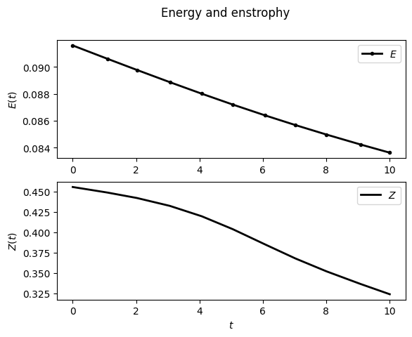
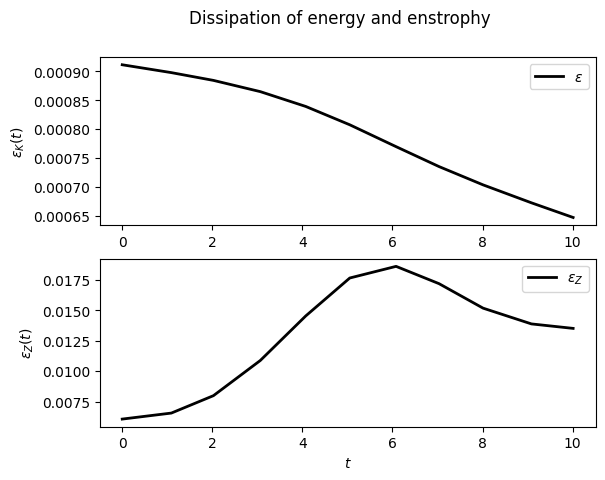
For example, to display the time evolution of spatially averaged quantities (here the energy, the entrophy and their dissipation rate):
sim.output.spatial_means.plot()
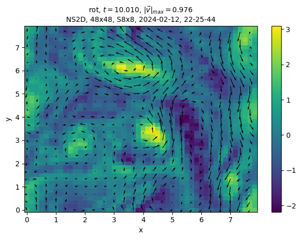
To plot the final state:
sim.output.phys_fields.plot()
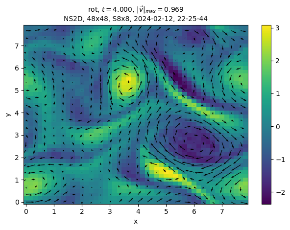
And a different time:
sim.output.phys_fields.plot(time=4)
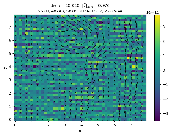
We can even plot variables that are not in the state in the solver. For example, in this solver, the divergence, which should be equal to 0:
sim.output.phys_fields.plot("div")
Finally we remove the directory of this example simulation…
shutil.rmtree(sim.output.path_run)